Summary
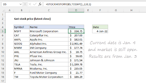
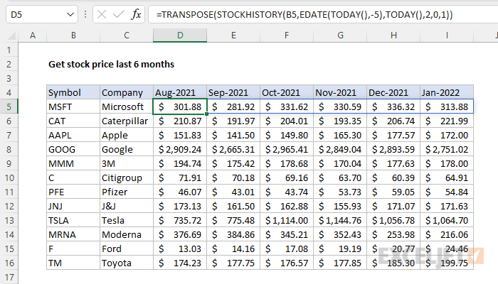
To get the monthly closing stock price over the past n months (i.e. last 6 months, last 12 months, last 24 months, etc.) you can use a formula based on the STOCKHISTORY function. In the example shown, the formula in cell D5, copied down, is:
=TRANSPOSE(STOCKHISTORY(B5,EDATE(TODAY(),-5),TODAY(),2,0,1))
The result is the monthly close price for each symbol listed in column B over the past 6 months. Note that STOCKHISTORY returns an array of values that spill onto the worksheet into multiple cells. The STOCKHISTORY is only available in Excel 365.
Generic formula
=TRANSPOSE(STOCKHISTORY(A1,EDATE(TODAY(),-(n-1)),TODAY(),2,0,1))
Explanation
In this example, the goal is to get monthly closing stock price over the past n months (i.e. last 6 months, last 12 months, last 24 months, etc.) for the list of symbols that appear in column B. In addition, we want a rolling time period, that stays in sync with the current date. This can be done with the STOCKHISTORY function, whose purpose is to retrieve historical information for a financial instrument over time.
Basic example
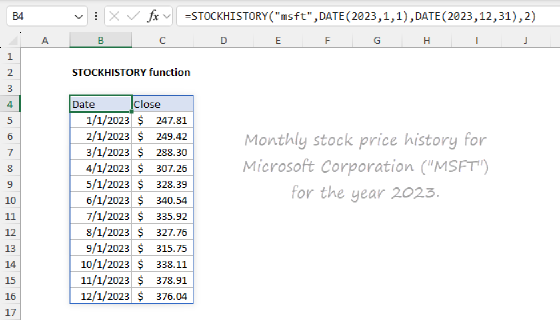
STOCKHISTORY retrieves historical stock price information for a given symbol and date range. STOCKHISTORY takes up to 11 arguments, most of which are optional. The syntax for the first 5 arguments looks like this:
=STOCKHISTORY(stock,start_date,[end_date],[interval],[headers])
The interval argument specifies the time period to use between prices. The options are daily (0), weekly (1), or monthly (2). In this case, we want a monthly interval, so we provide 2. For example, to retrieve the close price for Apple ("AAPL") for the last 6 months beginning in August 2022, we can use a formula like this:
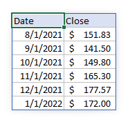
=STOCKHISTORY("AAPL","1-Aug-2021","1-Jan-2022",2)
The result is an array that includes headers, date, and close price:
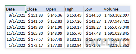
The remaining arguments (property1 to property5) specify the information STOCKHISTORY can return, which includes Date, Close, Open, High, Low, and volume. If we extend the formula to include all 6 properties, the formula looks like this:
=STOCKHISTORY("AAPL","1-Aug-2021","1-Jan-2022",2,,0,1,2,3,4,5)
And the result is an array with much more detail:
These properties can be reordered as desired by changing the order that the property numbers are listed. For example, to list Volume second, we can move Volume (5) to the second position after date (0):
=STOCKHISTORY("AAPL","1-Aug-2021","1-Jan-2022",2,,0,5,1,2,3,4)
For a more detailed overview of options, see our STOCKHISTORY function page.
Dynamic dates
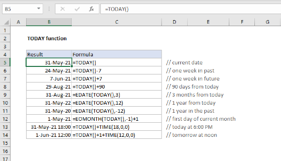
In the basic example above, the dates are hardcoded as text values. This works fine for a one-off formula, but in this case we want the formula to calculate the dates for us on an ongoing basis. We can do this by adding the TODAY function and the EDATE function to the formula. To calculate a start date 6 months in the past, we use the EDATE function like this:
=EDATE(TODAY(),-5) // date 6 months in the past
The TODAY function returns the current date directly to EDATE. If the date is January 8, 2021, EDATE returns the date August 8, 2021. To calculate the end_date, we use the TODAY() function by itself. Once we update the basic example above, we have a formula like this:
=STOCKHISTORY("AAPL",EDATE(TODAY(),-5),TODAY(),2)
The result is the same as before:
The difference is that this result will continue to update automatically as time goes by.
Note: There is no need to supply a first of month or last of month date to STOCKHISTORY. When interval is set to monthly (2), the STOCKHISTORY function will use the last close price for a date that lands anywhere in the month. For complete months in the past, this will be the last trading day of the month. For months not yet complete, STOCKHISTORY will return the latest close price available.
Horizontal layout
In order to display the last 6 months for each symbol in column B, we need to rotate the vertical format that STOCKHISTORY outputs by default to a horizontal layout. Along with this change, we also need to remove the date field and suppress the header. To start off, we can use the TRANSPOSE function to transpose vertical to horizontal:
=TRANSPOSE(STOCKHISTORY("AAPL",EDATE(TODAY(),-5),TODAY(),2))
This flips the layout to horizontal:
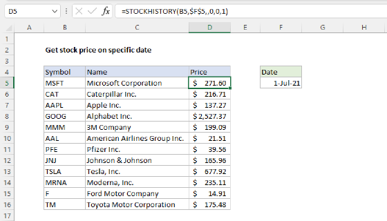
To remove Date and header, we need to adjust the value for header and customize properties. We use 0 for header and supply 1 for the first property to retrieve just the closing price. The formula now looks like this:
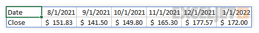
=TRANSPOSE(STOCKHISTORY("AAPL",EDATE(TODAY(),-5),TODAY(),2,0,1))
And the resulting array looks like this:
![]()
This is close to the final formula. To finalize, we just need to replace the hardcoded symbol "AAPL" with a reference to B5:
=TRANSPOSE(STOCKHISTORY(B5,EDATE(TODAY(),-5),TODAY(),2,0,1))
This is the formula used in cell D5, copied down the column.
The header
The last piece of the puzzle is the header. Note that we don't want a header that says "Date" or "Price". Instead, for each price that appears in a separate column, we want a header that shows a corresponding date. To keep things consistent, it would be nice if we could just adjust the arguments in STOCKHISTORY to return only a header, but this won't work; STOCKHISTORY will return a #VALUE error if only the date field is selected. As a workaround, we can adjust the formula to output both date and close price. First, we adjust the STOCKHISTORY function to remove only the header:
=TRANSPOSE(STOCKHISTORY(B5,EDATE(TODAY(),-5),TODAY(),2,0))
By default, STOCKHISTORY will return both Date and Price, so we no longer need to request the Price only, since we need the Dates. The result looks like this:
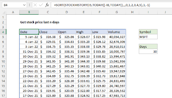
Next, we use the INDEX function to return just the first row of the array (the Dates):
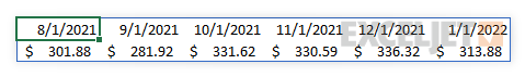
=INDEX(TRANSPOSE(STOCKHISTORY(B5,EDATE(TODAY(),-5),TODAY(),2,0)),1,0)
Inside INDEX, row_num is 1, and column_number is set 0, in order to return the entire row. The result is an array of dates that can be used as a header:
![]()
This is the formula used in D4 in the example. Note when interval is set to monthly (2), STOCKHISTORY will always show "first of month" dates. However, you can apply a custom date format to display the dates as you like. In the example shown, the date format used is "mmm-yyyy".