Summary
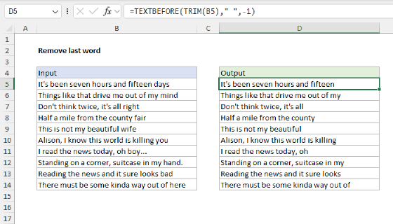
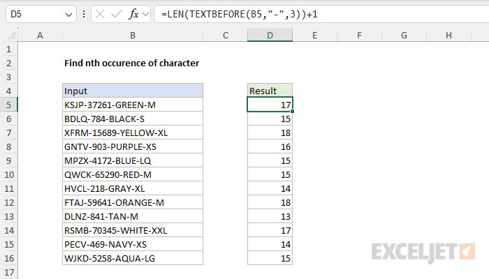
To find the nth occurrence of a character in a text string, you can use a formula based on the TEXTBEFORE function together with the LEN function. In the example shown, the formula in cell D5, copied down, is:
=LEN(TEXTBEFORE(B5,"-",3))+1
As the formula is copied down, it finds the position of the third occurrence of the hyphen (-) in each text string in column B.
Note: TEXTBEFORE is only available in newer versions of Excel. See below for a formula that will work in older versions.
Generic formula
=LEN(TEXTBEFORE(A1, delimiter, n))+1
Explanation
In this example, the goal is to determine the position of the nth occurrence of a specific character (delimiter) in the text strings in column B. This article explains two approaches:
- A modern formula based on the TEXTBEFORE function.
- A more traditional formula for older versions of Excel.
The first option is simpler, and you should use it if you have the TEXTBEFORE function in your version of Excel. The second formula is more complex and makes sense if you don't have TEXTBEFORE.
This formula is a great example of how new functions simplify previously complex Excel problems. The traditional formula is more complicated than the modern approach.
Introduction
When working with text strings, it's common to want to determine the location of a specific occurrence of a character. For example:
- The location of the third space (" ")
- The location of the second hyphen ("-")
- The location of the fourth slash ("/")
- And so on.
Once you know the position, you can feed it into other formulas to split the text string at that position or extract text before or after that position. For a long time, this has been a challenging problem in Excel because there has been no direct way to target, say, the third hypen ("-") in a text string. Functions like FIND and SEARCH are good at returning positions, but they cannot specify which instance of a character you want. They always find the first instance. The introduction of the TEXTBEFORE and TEXTAFTER functions in Excel is a big step forward because both functions provide an argument for instance number.
Modern formula based on TEXTBEFORE
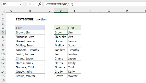
In the latest version of Excel, we can solve this problem easily using the TEXTBEFORE function. TEXTBEFORE extracts text that appears before a specified delimiter with a syntax like this:
=TEXTBEFORE(text,delimiter,instance_num)
For example, we can extract "ABC" from "ABC-123-XYZ" by using - as the delimiter and specifying the first instance:
=TEXTBEFORE("ABC-123-XYZ", "-", 1) // returns "ABC"
The third argument, instance_num, determines which occurrence of the delimiter to target. By default, it is set to 1, meaning the first occurrence. If we provide a 2, TEXTBEFORE extracts text before that second occurrence:
=TEXTBEFORE("ABC-123-XYZ", "-", 2) // returns "ABC-123"
We can use this behavior to figure out the location of the nth occurrence of a character, by adding in the LEN function. The idea is:
- Use
TEXTBEFOREto extract everything before the nth occurrence of the delimiter. - Use
LENto count the length of this extracted text. - Add
1to get the exact position of the nth occurrence.
The final formula in formula in cell D5 looks like this:
=LEN(TEXTBEFORE(B5,"-",3))+1
TEXTBEFORE(B5, "-", 3): Extracts everything before the third-.LEN(...): Returns the length of this extracted text.+1: Gives the exact position of the next character (our target)
Finding the position of the 1st, 2nd, 3rd, and 4th occurrence
Since this formula is simple, it's easy to customize its behavior. To find a different occurrence of a character, simply change the instance number n and adjust the delimiter as needed. The generic version of the formula looks like this:
=LEN(TEXTBEFORE(A1,delimiter,n)) + 1
In the example below, we are using a variable number for n in column D and the delimiter is *. The formula in F5 is:
=LEN(TEXTBEFORE(B5,"*",D5))+1
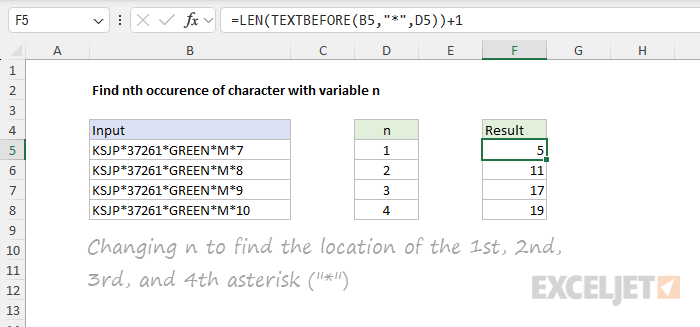
The result is the position of the first, second, third, and fourth asterisk ("*") in each text string.
Traditional formula for older versions of Excel
In older versions of Excel, finding the nth occurrence of a character is a bit more complicated because TEXTBEFORE is not available. Instead, we use the FIND and SUBSTITUTE functions together in a formula like this:
=FIND("~",SUBSTITUTE(B5,"-","~",3))
SUBSTITUTE is useful to us here because it has an optional instance_num argument that allows you to target the specific occurrence of the text you want to replace. We can't use this directly to find the nth occurrence of a character, but we can use it to replace the nth occurrence with a marker that we then locate with the FIND function. The formula works as follows:
SUBSTITUTE(B5, "-", "~", 3): Replaces the third-in the text with a unique marker (~).FIND("~", ...): Finds the position of this marker, which corresponds to the position of the third-in the original text.
This approach is effective but less intuitive than using TEXTBEFORE.
It's important that you use a unique marker that doesn't appear in the text string. In this case, we use the tilde character (~) , but you can adjust to suit your needs.
Customizing the traditional formula
The same formula structure can be used with a different delimiter. For example, to find the 4th *:
=FIND("~", SUBSTITUTE(A1, "*", "~", 4))
This allows you to locate any occurrence of a character in a text string.
Summary
- The new
TEXTBEFOREmethod is a bit simpler but requires a newer version of Excel. - The traditional
FIND+SUBSTITUTEmethod works well in older versions of Excel. - Both approaches allow customization by changing the delimiter and the instance number.