Explanation
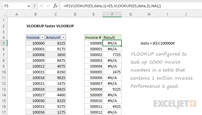
In this example, VLOOKUP is configured to look up 1000 invoice numbers in a table that contains 1 million invoices. The catch is that not all of the 1000 invoice numbers exist in the source data. In fact, most of the invoice numbers do not appear in column B. This means we need to configure VLOOKUP to use an exact match, and exact match lookups on large data sets can be painfully slow. However, because the data is sorted by invoice number, we can use the modified VLOOKUP formula seen in the worksheet. Although this formula uses VLOOKUP twice, it runs quickly.
Exact-match VLOOKUP is slow
When you use VLOOKUP in "exact match mode" on a large set of data, it can really slow down the calculation time in a worksheet. With very large sets of data, the calculation time can be minutes. To use VLOOKUP in exact match mode, provide FALSE or zero as the fourth argument, range_lookup:
=VLOOKUP(value,data,n,FALSE) // exact match
The reason VLOOKUP is slow in this mode is that there is no requirement that the lookup values be sorted. As a result, VLOOKUP must check every record in the data set until a match is found, or not. This is sometimes referred to as a linear search.
Approximate-match VLOOKUP is very fast
In approximate-match mode, VLOOKUP is extremely fast. To use approximate-match VLOOKUP, sort the data by the first column (the lookup column), then specify TRUE for range_lookup or omit the argument:
=VLOOKUP(value,data,n,TRUE) // approximate match
=VLOOKUP(value,data,n) // approximate match
With very large sets of data, changing to approximate-match VLOOKUP can mean a dramatic speed increase. This is because VLOOKUP will assume data is sorted and use a different algorithm to speed up searching, sometimes called a binary search.
For a complete VLOOKUP overview with many examples, see How to use VLOOKUP.
The problem
At first glance, a solution seems simple: sort the data, and use VLOOKUP in approximate match mode. However, the problem is that VLOOKUP won't return an error if a value is not found. Instead, it may return an incorrect result that looks completely normal. For example, in the worksheet shown, if we configure VLOOKUP to find the Amount for invoice 500010 with range_lookup set to TRUE, the result is 9225 even though invoice 500010 does not exist in the table:
=VLOOKUP(500010,data,2,TRUE) // returns 9225
This happens because VLOOKUP's behavior with approximate match enabled is "exact match or next smaller value". When VLOOKUP can't find invoice 500010, it matches the next smaller invoice number, which is 500008, and returns 9225. So, while the formula runs very quickly, the result is not reliable. Obviously, this is not something you want to explain to your boss.
A solution with VLOOKUP + VLOOKUP
One way to speed up VLOOKUP in this situation is to use VLOOKUP twice, both times in approximate match mode. This may seem counterintuitive because we are calling VLOOKUP twice. However, two fast operations are better than one slow operation. The trick is to structure the formula in a way that requires an exact match result. We do that by testing the result of the first VLOOKUP to see if did actually find the lookup value. In the worksheet shown, the formula in F5, copied down, is:
=IF(VLOOKUP(E5,data,1)=E5,VLOOKUP(E5,data,2),NA())
Notice the IF function controls the flow of the formula. If we do find the lookup value, we run the second lookup. Otherwise, we return an error. The logical_test inside the IF function looks like this:
VLOOKUP(E5,data,1)=E5
Here, we use VLOOKUP to find and return the lookup value itself, and we do so in approximate match mode by omitting the range_lookup argument. Remember, VLOOKUP defaults to an approximate match. Then we test the result against the lookup value. If this test returns TRUE, we know the lookup value exists in the data and we run the second VLOOKUP to fetch the desired value:
VLOOKUP(E5,data,2)
However, if the test returns FALSE, it means we didn't find the lookup value. In that case, we simply return an #N/A error with the NA function:
NA() // returns #N/A
To summarize: if we find the invoice number, we look up the amount. If we don't find an invoice number return #N/A error, which tells us the invoice number does not exist in the data. Even though the formula uses the VLOOKUP function two times, performance is good, because both instances of VLOOKUP use approximate match mode, which runs very quickly.
Summary
With large sets of data, exact match VLOOKUP can run painfully slow when configured for an exact match. This is because there is no requirement that the lookup values be sorted and VLOOKUP must perform a linear search, which is a slow operation when there are many values to check. On the other hand, if data is sorted, VLOOKUP can be configured for an approximate match by setting range_lookup to TRUE, or by omitting range_lookup altogether. In this configuration, VLOOKUP runs very fast. However, VLOOKUP may return an incorrect result. This happens because VLOOKUP's behavior with approximate match enabled is "exact match or next smaller value", so VLOOKUP matches the previous value when a match is not found. One way around this problem is to use VLOOKUP twice, both times in approximate match mode. The trick is to structure the formula in a way that leverages two fast lookups in a way that still ensures an exact match result.
Notes
- This approach is overkill unless lookup performance is an issue.
- Data must be sorted by lookup value in ascending order.
- The newer XLOOKUP function has a very fast binary search option.


