Summary
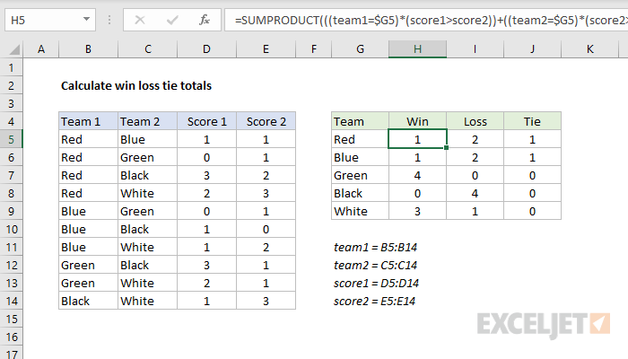
To calculate win, loss, and tie totals for a team using game data that includes a score for both teams, you can use a formula based on the SUMPRODUCT function. In the example shown, the formula in H5, copied down, is:
=SUMPRODUCT(((team1=$G5)*(score1>score2))+((team2=$G5)*(score2>score1)))
This formula returns total wins for the "Red" team based on the data shown, and uses these named ranges: team1 (B5:B14), team2 (C5:C14), score1 (D5:D14), and score2 (E5:E14).
Explanation
The goal in this example is to calculate total wins, losses, and ties for each team listed in column G. The problem is complicated somewhat by the fact that a team can appear in either column B or C, so we need to take this into account when calculating wins and losses. For convenience and readability only, the formula uses the following named ranges: team1 (B5:B14), team2 (C5:C14), score1 (D5:D14), and score2 (E5:E14).
In solving this problem, you might think of using the COUNTIF or COUNTIFS function, but these functions are limited to working with existing ranges for criteria. Instead, the formula in the example uses the SUMPRODUCT function to sum the result of an array expression based on Boolean logic. Inside SUMPRODUCT on the left we have an expression to count wins when a team appears in column B:
((team1=$G5)*(score1>score2))
If we replace the mixed reference $G5 with the value in G5, we have:
((team1="Red")*(score1>score2))
This expression is actually formed from two expressions, joined by multiplication (*) to create AND logic. The expression on the left checks if team1 is "Red":
(team1="Red") // check team is "Red"
The expression on the right checks if score1 is greater than score2:
(score1>score2) // check score1 greater than score2
Because both expressions involve ranges with multiple values, they each return arrays that contain multiple results. Rewriting the formula with the arrays returned, we have:
({TRUE;TRUE;TRUE;TRUE;FALSE;FALSE;FALSE;FALSE;FALSE;FALSE} *
{FALSE;FALSE;TRUE;FALSE;FALSE;TRUE;FALSE;TRUE;TRUE;FALSE})
The math operation of multiplication (*) works like AND in Boolean algebra and also coerces the TRUE and FALSE values into 1s and 0s. When corresponding values are both TRUE, the result is 1. In any other case, the result is 0. The result is a single array like this:
{0;0;1;0;0;0;0;0;0;0}
Note the third value is 1, which corresponds to game 3, where Red beats Black 3-2. At this point, we have collected an array that represents all Red victories when Red is Team1. This covers the left side of the logic inside SUMPRODUCT.
On the right side, we have similar logic that checks for Red wins when Read is Team2:
((team2=$G5)*(score2>score1))
This logic evaluates in the same way as the left logic. Summarized, we have:
((team2="Red")*(score2>score1))
Then:
({FALSE;FALSE;FALSE;FALSE;FALSE;FALSE;FALSE;FALSE;FALSE;FALSE})*({FALSE;TRUE;FALSE;TRUE;TRUE;FALSE;TRUE;FALSE;FALSE;TRUE})
Then:
({0;0;0;0;0;0;0;0;0;0})
Since Red doesn't actually appear as Team2 in any game, all results are zero.
With both the left and right sides evaluated, we can now rewrite the original formula like this:
=SUMPRODUCT(({0;0;1;0;0;0;0;0;0;0})+({0;0;0;0;0;0;0;0;0;0}))
At this point notice the math operator between the two arrays is addition (+), which corresponds to OR logic. We do this because we are counting Red wins as Team1 OR Team2. The result is a single array inside SUMPRODUCT:
=SUMPRODUCT({0;0;1;0;0;0;0;0;0;0})
With just one array to process, SUMPRODUCT sums the items in the array and returns a final result, 1.
For comparison, if we solve for the Green team in cell H7, we get 4:
=SUMPRODUCT(((team1=$G7)*(score1>score2))+((team2=$G7)*(score2>score1)))
Then:
=SUMPRODUCT(({0;0;0;0;0;0;0;1;1;0})+({0;1;0;0;1;0;0;0;0;0}))
Then:
=SUMPRODUCT({0;1;0;0;1;0;0;1;1;0}) // returns 4
Counting losses
The formula in I5 to count losses is very similar:
=SUMPRODUCT(((team1=$G5)*(score1<score2))+((team2=$G5)*(score2
The only difference is the "reversed" logic in checking scores.
Counting ties
The formula to count follows the same pattern, the only difference is we check for equal scores:
=SUMPRODUCT(((team1=$G5)*(score1=score2))+((team2=$G5)*(score2=score1)))
One problem with this formula is that games without scores are counted as ties. This happens because Excel evaluates empty cells as zero, so when score1 and score2 are empty, they appear to the formula as zero, which counts like a 0-0 tie. To work around this problem, you can add a second array to SUMPRODUCT to check for ties with logic based on the LEN function:
(LEN(score1)>0)*(LEN(score2)>0) // check for no score
When both score1 and score2 have values, the result is 1. When either score is empty, the result is zero, and this zero "cancels out" the false tie that occurs when both cells are empty. The complete formula is:
=SUMPRODUCT(
((team1=$G5)*(score1=score2))+
((team2=$G5)*(score2=score1)),
(LEN(score1)>0)*(LEN(score2)>0)
)
The LEN function is checking for any characters. When LEN returns zero, it means a cell is empty.