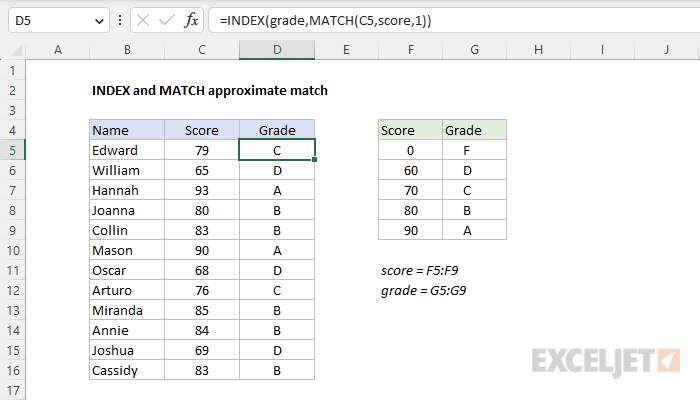
Explanation
In this example, the goal is to calculate the correct grade for each name in column B using the score in column C and the table to the right. For convenience only, grade (G5:G9) and score (F5:F9) are named ranges. This is a classic "approximate-match" lookup problem because it is unlikely that a score will be found in the lookup table. Instead, the table acts to group scores into buckets. For a given score, we want to match the largest value in the table that is less than or equal to the score. This problem can be solved with an INDEX and MATCH formula like this:
=INDEX(grade,MATCH(C5,score,1))
Background reading
This article assumes you are familiar with INDEX and MATCH. If not, see:
- How to use INDEX and MATCH - overview with simple examples
The MATCH function
The MATCH function locates a value in a set of data and returns its position. In this example, the formula uses MATCH to find the correct row for a given score. MATCH is configured to look for the value in C5 in the named range score (F5:F9):
MATCH(C5,score,1) // returns 3
Here, the lookup_value is the score in C5, the lookup_array is the named range score (F5:F9), and match_type is set to 1, for an approximate match. A match type of 1 will cause MATCH to find the first value in the table that is less than or equal to the lookup value in C5. In this case, the score is 79, so MATCH returns 3. Now that we have the correct row number, we need to retrieve the grade in that row. This is a job for the INDEX function.
The INDEX function
The INDEX function is designed to retrieve values at a known location. In this example, the MATCH function returns a result of 3 directly to the INDEX function as the row_num argument. Once MATCH returns 3 we can simplify the formula to:
=INDEX(grade,3) // returns "C"
With array provided as the named range grade (G5:G9) and a row number of 3, INDEX returns the value at the 3rd row in G5:G9, which is "C".
Note: For MATCH to work correctly with match_type of 1, the scores in F5:F9 must be sorted in ascending order. For more information, see our MATCH function page.


