XLOOKUP with logical criteria

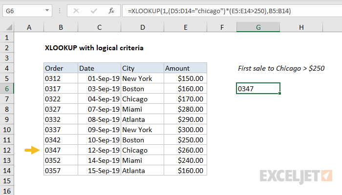
To use XLOOKUP with multiple logical, build expressions with boolean logic and then look for the number 1. In the example XLOOKUP is used to lookup the first sale to Chicago over $250. The formula in G6 is:

=XLOOKUP(1,(D5:D14="chicago")*(E5:E14>250),B5:B14)

which returns 0347, the order number of the first record that meets supplied criteria.

Note XLOOKUP is not case-sensitive.

How this formula works

XLOOKUP can handle arrays natively, which makes it a very useful function when constructing criteria based on multiple logical expressions.

In the example shown, we are looking for the order number of the first order to Chicago over $250. We are constructing a lookup array using the following expression and boolean logic:

(D5:D14="chicago")*(E5:E14>250)

When this expression is evaluated, we first get two arrays of TRUE FALSE values like this:

{FALSE;FALSE;TRUE;FALSE;FALSE;FALSE;FALSE;TRUE;FALSE;FALSE}*
{FALSE;FALSE;FALSE;TRUE;TRUE;TRUE;FALSE;TRUE;FALSE;FALSE}

When the two arrays are multiplied by one another, the math operation results in a single array of 1's and 0's like this:

{0;0;0;0;0;0;0;1;0;0}

We now have the following formula, and you can see why we are using 1 for the lookup value:

=XLOOKUP(1,{0;0;0;0;0;0;0;1;0;0},B5:B14)

XLOOKUP matches the 1 in 8th position, and returns the correponding 8th value from B5:B14, which is 0347.

With a single criteria

As seen above, math operations automatically coerce TRUE and FALSE values to 1's and 0's. Therefore, when using multiple expressions, a lookup value of 1 makes sense. In cases where you have only a single criteria, say, "amount > 250", you can look for TRUE instead like this:

=XLOOKUP(TRUE,E5:E14>250,B5:B14)

Alternatively, you can force the TRUE FALSE values to 1's and 0's, and use 1 like this.

=XLOOKUP(1,--(E5:E14>250),B5:B14)