Summary
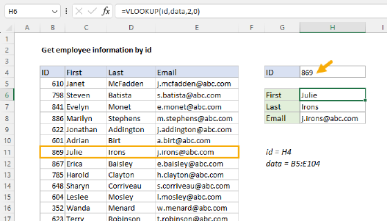
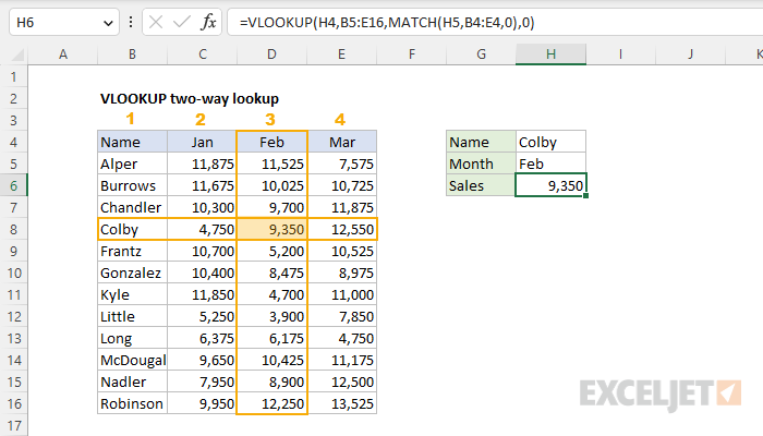
To perform a two-way lookup (i.e. a matrix lookup), you can combine the VLOOKUP function with the MATCH function to get a column number. In the example shown, the formula in cell H6 is
=VLOOKUP(H4,B5:E16,MATCH(H5,B4:E4,0),0)
Cell H4 provides the lookup value for the row ("Colby"), and cell H5 supplies the lookup value for the column ("Feb". The result is 9,350, the value for Colby in February.
Generic formula
=VLOOKUP(value,table,MATCH(value,range,0),0)
Explanation
In this example, the goal is to perform a two-way lookup based on the name in cell H4 and the month in cell H5 with the VLOOKUP function. Inside the VLOOKUP function, the column index argument is normally hard-coded as a static number. However, you can create a dynamic column index number by using the MATCH function to locate the right column. This technique allows you to create a dynamic two-way lookup, matching on both rows and columns. It can also make a VLOOKUP formula more resilient. VLOOKUP can break when columns are inserted or removed from a table, but a formula that uses VLOOKUP + MATCH can continue to work correctly even changes are made to columns.
VLOOKUP formula
This is a standard VLOOKUP exact match formula with one exception: the column index is supplied by the MATCH function. If we remove the MATCH function, the core VLOOKUP formula to match the name in H4 and retrieve a value for February is:
=VLOOKUP(H4,B5:E16,3,0)
The lookup_value is the name in cell H4, the table_array is the range B5:E16, the col_index_num is hardcoded as 3 (to retrieve values from the "Feb" column), and range_lookup is set to 0 to force an exact match. (Note: you can use either zero or FALSE for range_lookup with the same result). With these inputs, the formula returns 9,350, the value for Colby in February.
MATCH formula
The goal in this example is to dynamically generate a column number for VLOOKUP based on the value in cell H5. To do this, we use the MATCH function like this:
MATCH(H5,B4:E4,0) // returns 3
The lookup_value is the month abbreviation in cell H5, the lookup_array is the range B4:E4, and match_type is set to zero (0) to specify an exact match. With this configuration, MATCH returns 3 since the matching value is in cell D4, which is the third value in the range B4:E4. Note that the lookup array given to MATCH (BB4:E4) representing column headers deliberately includes cell B4, even though cell B4 does not contain a month name. This is done so that the number returned by MATCH is in sync with the lookup table given by VLOOKUP. In other words, we need to give MATCH a range that spans the same number of columns as the lookup table given to VLOOKUP.
VLOOKUP + MATCH
The final formula with VLOOKUP and MATCH together is:
=VLOOKUP(H4,B5:E16,MATCH(H5,B4:E4,0),0)
Notice that the MATCH function is provided to VLOOKUP as the column index number. Excel evaluates the formula from the inside out. The MATCH function is evaluated and returns 3 directly to VLOOKUP as col_num_index:
=VLOOKUP(H4,B5:E16,3,0)
The VLOOKUP function then runs and returns a final result of 9,350. This is the value for Colby in February. Note that the month lookup is now dynamic. For example, if the month is changed to "Mar", MATCH returns 4 and VLOOKUP returns a final result of 12,550.