VLOOKUP variable commission split

To calculate a commission, and split the Commission between Agent and Broker according to a variable schedule, you can use the VLOOKUP function. In the worksheet shown, the formula in D5 is:

=C5*VLOOKUP(B5,split,2,TRUE)

Where split is the named range G7:I11 The result in cell D5 is 7,500, based on a 3% commission calculated at 15,000, and a split of 50/50 between the Agent and Broker.

Explanation

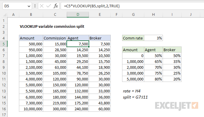
In this example, the goal is to calculate the correct commission for both Agent and Broker based on a 3% commission which is split according to the table in G7:I11, which is named split. Notice the amount going to the Agent and Broker changes as the total amount increases, which the Agent getting a larger share for higher amounts. The example assumes all commissions are 3%, as set in cell H4, the named range rate. This is a nice example of how the result from VLOOKUP can easily be used inside another formula.

Total commission

The total commission amount is calculated in cell C5 with this formula:

=B5*rate // total commission

Where rate is the named range H4. As the formula is copied down, a total commission is calculated for each amount in column B. If the commission rate in H4 is changed, all amounts will update.

Agent and Broker split

The Agent and Broker portion of the total commission shown in columns D and E are calculated like this:

=C5*VLOOKUP(B5,split,2,TRUE) // agent
=C5*VLOOKUP(B5,split,3,TRUE) // broker

Notice these formulas are identical except for the column index. The formula for Agent returns a value from column 2 in the table, and the formula for Broker returns a value from column 3 in the table. In both formulas, VLOOKUP is set to approximate match explicitly, by setting the optional fourth argument, range_lookup, to TRUE.

Note: When doing an approximate match, VLOOKUP assumes the table is sorted in ascending order. If VLOOKUP finds an exact match, it returns a value from the matching row. If VLOOKUP encounters a value greater than the lookup value, it will return a value from the previous row.