Two-way lookup VLOOKUP in a Table

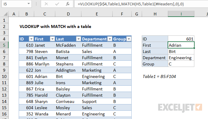
To do a two-way lookup in an Excel Table, you can use the MATCH function with a structured reference and VLOOKUP. In the example shown, the formula in I5 (copied down) is:

=VLOOKUP($I$4,Table1,MATCH(H5,Table1[#Headers],0),0)

Explanation

At a high level, we using VLOOKUP to extract employee information in 4 columns with ID as the lookup value. The ID value comes from cell I4, and is locked so that it won't change as the formula is copied down the column.

The table array is the table named Table1, with data in the range B5:F104.

The column index is provided by the MATCH function.

And match type is zero, so force VLOOKUP to perform an exact match.

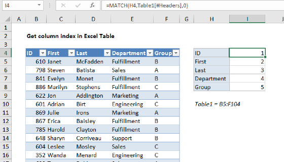
The MATCH function is used to get a column index for VLOOKUP like this:

MATCH(H5,Table1[#Headers],0)

This is what accomplishes the two-way match. Values in column H correspond to the headers in the table, so these go into match as lookup values.

The array is the headers in Table1, specified as a structured reference.

Match type is set to zero to force an exact match.

MATCH then returns the position of the match. For the formula in I5, this the position is 2, since "First" is the second column in the table.

VLOOKUP then returns the first name for id 601, which is Adrian.

Note: VLOOKUP depends on the lookup value being to the left of the value being retrieved in a table. Generally, this means the lookup value will be the first value in the table. If you have data where the lookup value is not the first column, you can switch to INDEX and MATCH for more flexibility.