Get column index in Excel Table

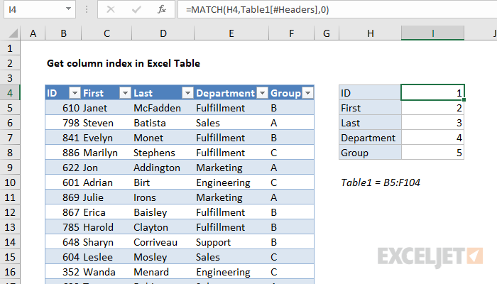
To get the index of a column in an Excel Table, you can use the MATCH function. In the example shown, the formula in I4 is:

=MATCH(H4,Table1[#Headers],0)

When the formula is copied down, it returns an index for each column listed in column H. Getting an index like this is useful when you want to refer to table columns by index in other formulas, like VLOOKUP, INDEX and MATCH, etc.

Explanation

This is a standard MATCH formula where the lookup values come from column H, the array is the headers in Table1, and match type is zero, to force an exact match.

The only trick to the formula is the use of a structured reference to return a range for the table headers to the MATCH function:

Table1[#Headers]

The nice thing about this reference is that it will automatically adjust to any changes in the table. Even when columns are added or removed, the reference will continue to return the correct range.