Excel formula: SUMIFS with horizontal range

Summary

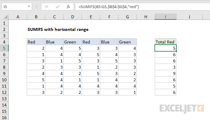
To use SUMIFS with a horizontal range, be sure both the sum range and criteria range are the same dimensions. In the example shown, the formula in cell I5 is:

=SUMIFS(B5:G5,$B$4:$G$4,"red")

which returns the total of items in "Red" columns for each row.

Explanation

Normally, SUMIFS is used with data in a vertical arrangement, but it can also be used in cases where data is arranged horizontally. The trick is to make sure the sum range and criteria range are the same dimensions. In the example shown, the formula in cell I5, copied down the column is:

=SUMIFS(B5:G5,$B$4:$G$4,"red")

Notice the criteria range, B4:G4 is locked as an absolute reference to prevent changes as the formula is copied.

Totals for each color

By carefully using a combination of absolute and mixed references, you can calculate totals for each color in a summary table. Notice in the example below, we are now picking up the cell references, I4, J4, and K4 to use directly as criteria:

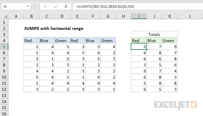
SUMIFS horizontal range to subtotal rows

The formula below in cell I5, copied down and across the table is:

=SUMIFS($B5:$G5,$B$4:$G$4,I$4)

Notice references are set up carefully so that the formula can be copied across and down:

The sum range, $B5:$G5, is a mixed reference with columns locked
The criteria range, B$4:$G$4 is absolute and fully locked as before
The criteria is a mixed reference, I$4, with the row locked

Author

Dave Bruns

Related formulas

Sum entire column

Excel supports "full column" and "full row" references like this: = SUM ( A:A ) // sum all of column A = SUM ( 3 : 3 ) // sum all of row 3 You can see how this works yourself by typing "A:A", "3:3", etc. into the name box (left of the formula bar)...

Sum matching columns

At the core, this formula relies on the SUMPRODUCT function to sum values in matching columns in the named range "data" C5:G14. If all data were provided to SUMPRODUCT in a single range, the result would be the sum of all values in the range: =...

Related functions

Excel SUMIFS Function

SUMIFS is a function to sum cells that meet multiple criteria. SUMIFS can be used to sum values when adjacent cells meet criteria based on dates, numbers, and text. SUMIFS supports logical operators (>,...

Excel Formula Training

Formulas are the key to getting things done in Excel. In this accelerated training, you'll learn how to use formulas to manipulate text, work with dates and times, lookup values with VLOOKUP and INDEX & MATCH, count and sum with criteria, dynamically rank values, and create dynamic ranges. You'll also learn how to troubleshoot, trace errors, and fix problems. Instant access. See details here.