Summary
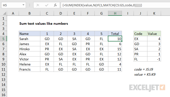
To translate text values into numbers and sum the result, you can use an INDEX and MATCH formula, and the SUM function. In the example shown, the formula in H5 is:
{=SUM(INDEX(value,N(IF(1,MATCH(C5:G5,code,0)))))}
where "code" is the named range K5:K9, and "value" is the named range L5:L9.
Note: this is an array formula, and must be entered with control + shift + enter.
Explanation
The heart of this formula is a basic INDEX and MATCH formula, used to translate text values into numbers as defined in a lookup table. For example, to translate "EX" to the corresponding number, we would use:
=INDEX(value,MATCH("EX",code,0))
which would return 4.
The twist in this problem however is that we want to translate and sum a range of text values in columns C through G to numbers. This means we need to provide more than one lookup value, and we need INDEX to return more than one result. The standard approach is a formula like this:
=SUM(INDEX(value,MATCH(C5:G5,code,0)))
After MATCH runs, we have an array with 5 items:
=SUM(INDEX(value,{2,2,3,2,5}))
So it seems INDEX should return 5 results to SUM. However, if you try this, the INDEX function will return only one result SUM. To get INDEX to return multiple results, we need to use a rather obscure trick, and wrap MATCH in N and IF like this:
N(IF(1,MATCH(C5:G5,code,0)))
This effectively forces INDEX to provide more than one value to the SUM function. After INDEX runs, we have:
=SUM({3,3,2,3,-1})
And the SUM function returns the sum of items in the array, 10. For a good write up on this behavior, see this article by Jeff Weir on the StackOverflow site.