Summary
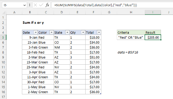
To sum numbers based on multiple criteria, you can use the SUMIFS function. In the example shown, the formula in I6 is:
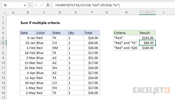
=SUMIFS(F5:F16,C5:C16,"red",D5:D16,"tx")
The result is $88.00, the sum of the Total in F5:F16 when the Color in C5:C16 is "Red" and the State in D5:D16 is "TX". Note that the SUMIFS function is not case-sensitive.
Generic formula
=SUMIFS(sum_range,range1,criteria1,range2,criteria2)
Explanation
In this example, the goal is to sum the values in F5:F16 when the Color in C5:C16 is "Red" and the State in D5:D16 is "TX". This is an example of a conditional sum with multiple criteria and the SUMIFS function is the easiest way to solve this problem.
SUMIFS function
The SUMIFS function sums cells in a range that meet one or more conditions, referred to as criteria. To apply criteria, the SUMIFS function supports logical operators (>,<,<>,=) and wildcards (*,?) for partial matching. The syntax for the SUMIFS function depends on the number of conditions needed. Each separate condition will require a range and a criteria. The generic syntax for SUMIFS looks like this:
=SUMIFS(sum_range,range1,criteria1) // 1 condition
=SUMIFS(sum_range,range1,criteria1,range2,criteria2) // 2 conditions
The first argument, sum_range, is the range of cells to sum, which should contain numeric values. Notice the conditions (called criteria) are entered in pairs. Each new condition requires a separate range and criteria.
Example - Red and TX
We start off with sum_range, which is the range F5:F16:
=SUMIFS(F5:F16,
Next, we add the first condition, which is that the Color in C5:C16 is "Red":
=SUMIFS(F5:F16,C5:C16,"red"
The range is C5:C16, and the criteria is "red". Note that SUMIFS is not case-sensitive, so "red" will match "Red", "RED", and "red". Next, we need to add the second condition, which is that the State in D5:D16 is "TX". Again, we need to supply both a range and a criteria:
=SUMIFS(F5:F16,C5:C16,"red",D5:D16,"tx")
When the formula is entered, the result is $88.00, the sum of the Total in F5:F16 when the Color in C5:C16 is "Red" and the State in D5:D16 is "TX".
Example - Red and >20
Next, the goal is to sum the Total in F5:F16 when the color is "red" and the value of Total is greater than $20. This means we need to include the logical operator (>) in the second criteria. The formula in I7 is:
=SUMIFS(F5:F16,C5:C16,"red",F5:F16,">20")
To read more about the syntax needed to apply logical operators and use wildcards with the SUMIFS function, see this page.