Explanation
At the core, the OFFSET function delivers a range of 3 cells to SUM, which returns a summed result.
The arguments for OFFSET are provided as follows:
For reference we use the first cell in the data range, B5, entered as a mixed reference (column locked, row relative).
For rows, we use 0, since we don't need to change rows.
For cols, we use the expression:
(COLUMN()-COLUMN($O$5))*3
This part of the formula figures out how many columns from the starting reference to offset. In O5, the offset is zero, in P5, the offset is 3, and so on.
Finally, height is input as 1 and width is input as 3, since in this case we always want a 1 x 3 range of cells.
Note: change 3 to the multiplier you need, shown as "n" in the generic form of the formula above.


