Summary
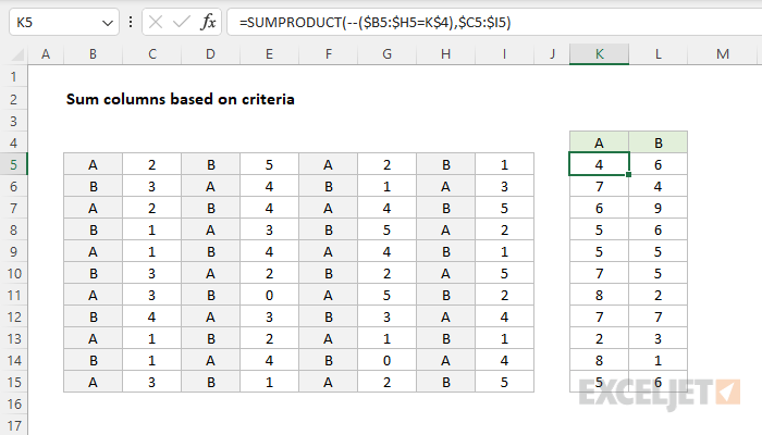
To sum values in columns based on criteria in an adjacent column, you can use a formula based on the SUMPRODUCT function. In the example shown, the formula in K5 is:
=SUMPRODUCT(--($B5:$H5=J$4),$C5:$I5)
As the formula is copied across and down, it returns a sum of values associated with "A" and "B" in the table to the left.
Generic formula
=SUMPRODUCT(--(range1=criteria),range2)
Explanation
In this example, the goal is to sum the values in columns C, E, G, and I conditionally using the text values in columns B, D, F, and H for criteria. This problem can be solved with the SUMPRODUCT function, which is designed to multiply ranges or arrays together and return the sum of products. The formula in K5 is:
=SUMPRODUCT(--($B5:$H5=K$4),$C5:$I5)
Working from the inside out, SUMPRODUCT is configured with two arguments, array1 and array2. The first array, array1, is set up to act as a "filter" to allow only values that meet criteria:
--($B5:$H5=K$4)
Note: both references above are mixed references. $B5:$H5 has the columns locked, so that the formula can be copied across. K$4 has the row locked so that the formula can be copied down.
All values in the range B5:H5 are compared to the value in K4. The result is an array of TRUE and FALSE values like this:
{TRUE,FALSE,FALSE,FALSE,TRUE,FALSE,FALSE}
In this array, each TRUE value corresponds to the value "A" in B5:H5, and FALSE values correspond to other values. The double negative (--) is used to convert the TRUE and FALSE values to 1s and 0s and the result looks like this:
{1,0,0,0,1,0,0}
We can now simplify the formula like this:
=SUMPRODUCT({1,0,0,0,1,0,0},$C5:$I5)
The second array, input as $C5:$I5, evaluates to:
{2,"B",5,"A",2,"B",1}
We can now simplify the formula to:
=SUMPRODUCT({1,0,0,0,1,0,0},{2,"B",5,"A",2,"B",1})
Next, SUMPRODUCT multiplies the two arrays together. Only the values in the second array that correspond to 1s in the first array survive this operation. Since SUMPRODUCT is programmed to ignore the errors that result from multiplying text values, the final array looks like this:
{2,0,0,0,2,0,0}
SUMPRODUCT then sums the array and returns a final result of 4.
=SUMPRODUCT({2,0,0,0,2,0,0}) // returns 4
This represents the numbers that correspond to "A'" in row 5. As the formula is copied down and across, we get a sum for "A" and "B" in each row.