Summary
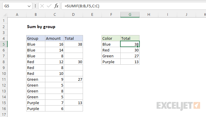
To sum data by group you can use the SUMIF function or the SUMIFS function. In the example shown, the formula in G5 is:
=SUMIF(B:B,F5,C:C)
With "Blue" in cell F5, the result is 38. As the formula is copied down, it returns a count of each color listed in column F. See below for an explanation of the formula in column D.
Generic formula
SUMIF(A:A,A1,B:B)
Explanation
In this example, the goal is to sum by group, where each group is represented by a different color: Blue, Red, Green, and Purple. The worksheet shown contains two different approaches. In the range F5:G8, we have created a summary table to summarize counts by color. In column D, we are using a modified formula that reports a total per group the first time the group appears in the data. The article below explains both approaches.
Note: both formulas below use full column references (e.g. B:B, C:C). Full column references are a compact way to express a formula, and they automatically pick up new data in a column. However, they can also cause performance problems in some formulas, and they can return incorrect results when they intersect data elsewhere in a worksheet . In general, an Excel Table or a dynamic named range is a safer way to refer to data that may shrink or grow. All that said, you will run into full column references in worksheets developed by others, so it is important to understand how they work.
Summary table
One approach to solving this problem is to create a summary table to summarize results by group, as seen in the range F5:G8. The solution relies on the SUMIF function. The formula in G5, copied down, is:
=SUMIF(B:B,F5,C:C)
In this formula, B:B is the range, F5 is the criteria, and C:C is the sum_range. As the formula is copied down the column, the reference to F5 changes at each new row while the full column references do not change. The result is a subtotal by group of the amounts in column C.
Note: in the latest version of Excel, new functions make it possible to create summary tables that automatically update to include new groups. See this example for details.
Inline totals
Another way to approach this problem is to perform the calculations directly in the data in column D as seen in the worksheet. The formula in cell D5, copied down, is:
=IF(B5=B4,"",SUMIF(B:B,B5,C:C))
In this formula, we use the IF function to test each value in column B to see if its the same as the previous value (i.e. the cell above). If the two values match, we return an empty string (""). If the values do not match, the IF function returns this SUMIF formula:
SUMIF(B:B,B5,C:C)
This formula works the same way as the formula used in the summary table. As the formula is copied down the column, the reference to B5 changes at each new row while the full column references do not change. Because the IF function is suppressing the SUMIF formula when the values in column B match, the sums only appear in column D the first time a new color is encountered.
Note: this formula depends on data being sorted by group in order to get sensible results. One advantage of the summary table approach is that the sort order doesn't matter.
Performance
As mentioned earlier, full column references can cause performance problems in some cases, because worksheets in Excel contain more than 1 million rows. Excel does try to limit calculations to the "used range" of a worksheet, in order to reduce the number of calculations being performed. However, be aware that full column references can cause severe performance problems in specific circumstances. Charles Williams over at Fast Excel has a good article on this topic, with a full set of timing results.
Why about Pivot Tables?
Pivot tables remain an excellent way to group and summarize data.