Summary
To subtotal values by cell color you can use a few different approaches. In the example shown above, the formula in G5 to count amounts that are highlighted in green is:
=COUNTIF(amount,F5)
where color (D5:D16) and amount (C5:C16) are named ranges. This is an indirect approach that works because the logic that has been used to apply color is easily reproducible inside the COUNTIF function. See below for a more direct approach.
Explanation
In this example, the goal is to subtotal (count and sum) values based on cell color. This is a tricky problem, because there is no Excel function that will let you count cells by color directly. There are several different approaches, as explained below.
Standard formula logic
If color is being applied based on specific rules (either with conditional formatting or manually) you may be able to use standard logic that follows the same rules to count and sum by color. This is an indirect way to solve this problem because the formula is not actually checking cell color but is instead applying logic that mirrors the rules that were used to apply the color. However, it is a simple and clean way to solve the problem in compatible scenarios.
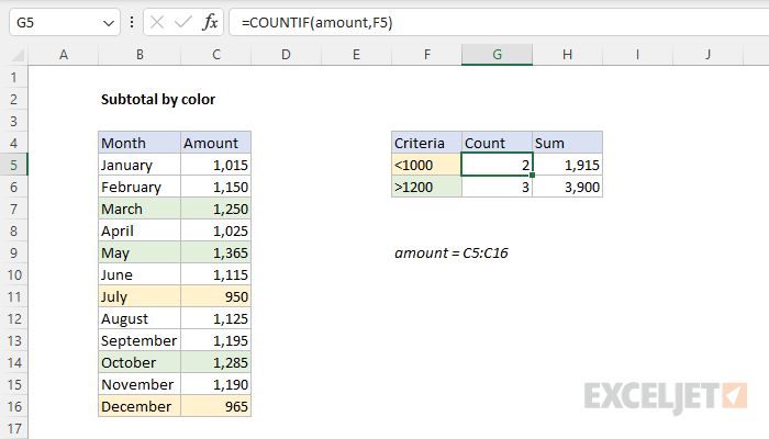
In the screen below, the green and yellow color is applied with two separate conditional formatting rules. When a value in column C is less than 1000, yellow formatting is applied. When a value is greater than 1200, green formatting is applied. The formulas in G5:G6, and H5:H6 use this same criteria to count and sum the data. The formula in cell G5 is:
=COUNTIF(amount,F5)
=COUNTIF(C5:C16,"<1000") // returns 2
The formula in H5 is:
=SUMIF(amount,F5)
=SUMIF(C5:C16,"<1000") // returns 1915
This approach only works in cases where cell color is being applied with rules that can be applied in a formula. It won't handle cases where color is applied to cells randomly, or in a way that can't be mimicked in a formula. For that situation, see the GET.CELL option below.
GET.CELL function
In cases where cell color has been applied manually (i.e. not with conditional formatting), you can use an obscure function called GET.CELL to retrieve cell color as a numeric code, then use this code to calculate the subtotals you need, as seen in the worksheet below:
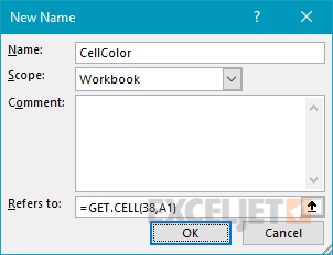
GET.CELL can't be used in a formula directly, you must first create a named range that uses GET.CELL to get the color of the cell directly to the left. To do this, place the cursor in cell B1, then create a new named range called "CellColor" that refers to cell A1 like this:
=GET.CELL(38,A1)
Another option to define a cell "one column to the left in the same row" is to use an R1C1-style reference with the INDIRECT function like this:
=GET.CELL(38,INDIRECT("RC[-1]",FALSE))There is very little good documentation on GET.CELL, but I did find this interesting 20+ year old link on MrExcel.com that provides a list of available arguments.
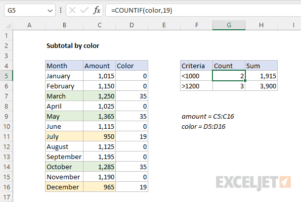
Because we are using relative references, this essentially means: get the color code of the cell directly to the left. Once you have defined the named range, you can use it in a column directly to the right of the cell you want color information for. In the worksheet shown below, CellColor is used in cell D5 like this:
=CellColor
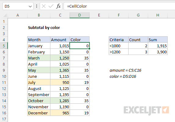
In cases where the cell to the left does not have a fill color, the result is zero (0). In cases where a fill color has been applied, CellColor will return a unique numeric code for that particular color. In the example shown, light green is 35 and light yellow is 19. In cell G5, the formula is:
=COUNTIF(color,19) // returns 2
where color is the named range D5:D16. Notice we are hardcoding 19 into the formula to count cells that have a light yellow fill. In cell G6, we count the colors that are 35 (light green):
=COUNTIF(color,35) // returns 3
The formulas in cells H5 and H6 use SUMIF to sum amounts based on the same color codes:
=SUMIF(color,19,amount) // returns 1915
=SUMIF(color,35,amount) // returns 3900
where color (D5:D16) and amount (C5:C16) are named ranges.
Note: the GET.CELL function is an old macro-based function. You will need to save your worksheet with macros enabled (i.e. with the extension .xlsm) to use it.
With a filter and SUBTOTAL
Another way to solve this problem is to use Excel's "Filter by Color" feature with the SUBTOTAL function. To take this approach, first enable a filter on the data you are working with like this:
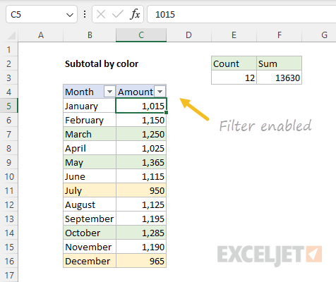
Next, either above or below the data, enter the SUBTOTAL function configured to target visible cells. In the screen below, the formulas to count and sum visible cells are:
=SUBTOTAL(102,amount) // count visible
=SUBTOTAL(109,amount) // sum visible
where amount is the named range C5:C16. The function_num 102 directs SUBTOTAL to count visible cells, and the number 109 tells SUBTOTAL to sum visible cells. Finally, select a target color in the Filter by Color menu:
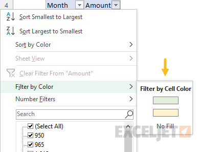
Filtering by color will exclude rows that do not match the target color and the SUBTOTAL formulas entered previously will show results that apply only to the color selected:
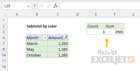
To show results for another color, just change the target color in the Filter by Color menu.
Note: Another way to solve this problem is to create a custom function with VBA. Sumit Bansal has a good summary of this approach here.