Self-contained VLOOKUP

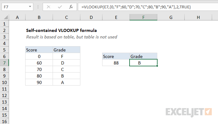
To make a self-contained VLOOKUP formula, you can convert the table to an array constant inside of VLOOKUP. In the example shown, the formula in F7 is:

=VLOOKUP(E7,{0,"F";60,"D";70,"C";80,"B";90,"A"},2,TRUE)

How this formula works

Normally, the second argument for VLOOKUP is provided as a range like B6:C10. When the formula is evaluated, this reference is converted internally to two dimensional array like this:

{0,"F";60,"D";70,"C";80,"B";90,"A"}

Each comma indicates a column, and each semi-colon indicates a row. Knowing this, when a table is small, you can convert the table to an "array constant" and use the array constant inside VLOOKUP, instead of the reference.

The advantage is that you no longer need to maintain a table on the worksheet. The disadvantage is that the array is hard-coded into the formula. If you copy the formula to more than one cell, you will have to maintain more than one instance of the array. Editing an array constant is more difficult than editing a table on the worksheet, and other users may not understand the formula.

Named range option

If you want a self-contained table, but don't want multiple instances of the table in the worksheet, you can create a named range using the array constant, then refer to the the named range in VLOOKUP. The advantage of this approach is that there is only once instance of the table to maintain.