Summary
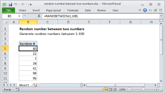
To generated a random number, weighted with a given probability, you can use a helper table together with a formula based on the RAND and MATCH functions.
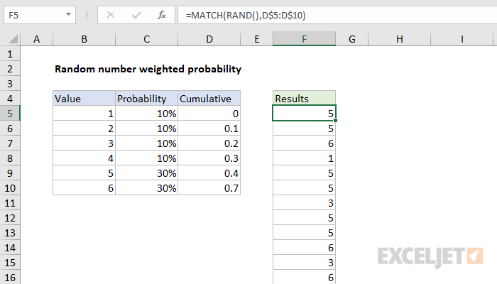
In the example shown, the formula in F5 is:
=MATCH(RAND(),D$5:D$10)
Generic formula
=MATCH(RAND(),cumulative_probability)
Explanation
This formula relies on the helper table visible in the range B4:D10. Column B contains the six numbers we want as a final result. Column C contains the probability weight assigned to each number, entered as a percentage. Column D contains the cumulative probability, created with this formula in D5, copied down:
=SUM(D4,C4)
Notice, we are intentionally shifting the cumulative probability down one row, so that the value in D5 is zero. This is to make sure MATCH is able to find a position for all values down to zero as explained below.
To generate a random value, using the weighted probability in the helper table, F5 contains this formula, copied down:
=MATCH(RAND(),D$5:D$10)
Inside MATCH, the lookup value is provided by the RAND function. RAND generates a random value between zero and 1. The lookup array is the range D5:D10, locked so it won't change as the formula is copied down the column.
The third argument for MATCH, match type, is omitted. When match type is omitted, MATCH will return the position of the largest value less than or equal to the lookup value*. In practical terms, this means the MATCH function travels along the values in D5:D10 until a larger value is encountered, then "steps back" to the previous position. When MATCH encounters a value larger than the largest last value in D5:D10 (.7 in the example), it returns the last position (6 in the example). As mentioned above, the first value in D5:D10 is deliberately zero to ensure that values below .1 are "caught" by the lookup table and return a position of 1.
*Values in the lookup range must be sorted in ascending order.
Random weighted text value
To return a random weighted text value (i.e. a non-numeric value), you can enter text values in the range B5:B10, then add INDEX to return a value in that range, based on the position returned by MATCH:
=INDEX($B$5:$B$10,MATCH(RAND(),D$5:D$10))
Notes
- I ran into this approach in a forum post on mrexcel.com
- RAND is a volatile function and will recalculate with every worksheet change
- Once you have random value(s), use paste special > values to replace the formula if needed