Summary
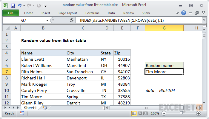
To get a random value from a table or list in Excel, you can use the INDEX function with help from the RANDBETWEEN and ROWS functions.
In the example shown, the formula in G7 is:
=INDEX(data,RANDBETWEEN(1,ROWS(data)),1)
Generic formula
=INDEX(data,RANDBETWEEN(1,ROWS(data)),1)
Explanation
Note: this formula uses the named range "data" (B5:E104) for readability and convenience. If you don't want to use a named range, substitute $B$5:$E$104 instead.
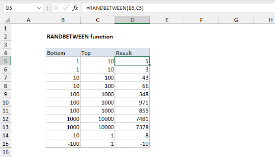
To pull a random value out of a list or table, we'll need a random row number. For that, we'll use the RANDBETWEEN function, which generates a random integer between two given values - an upper value and lower value.
For the lower value, we use the number 1, and for the upper value we use the ROWS function to get count the total rows in the table or list:
=RANDBETWEEN(1,ROWS(data))
RANDBETWEEN will return a random number between 1 and the count of rows in the data, and this result is fed into the INDEX function for the rows argument. For the columns argument, we simply use 1, since we want a name from the first column.
So, assuming that RANDBETWEEN returns 7 (as in the example) the formula reduces to:
=INDEX(data,7,1)
Which returns the name "Tim Moore", in row 7 of the table.
Note that RANDBETWEEN will recalculate whenever a worksheet is changed or opened.