Summary
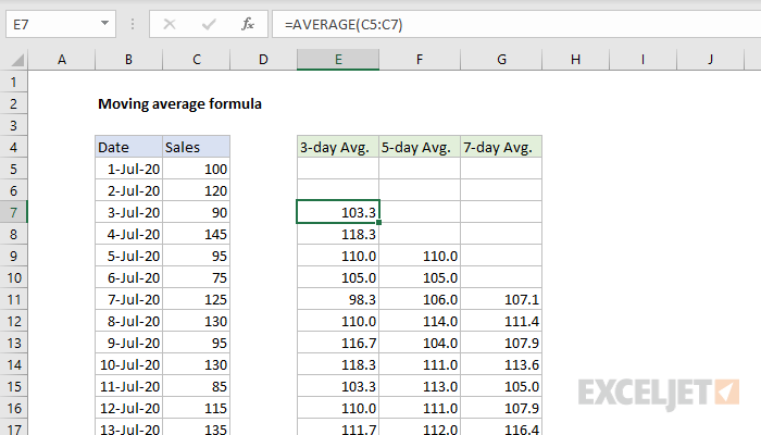
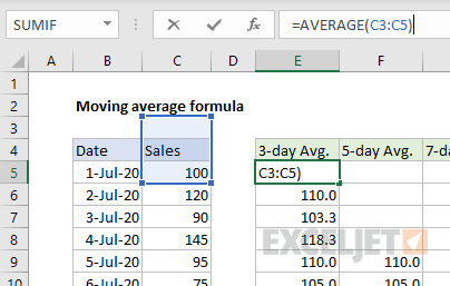
To calculate a moving or rolling average, you can use a simple formula based on the AVERAGE function with relative references. In the example shown, the formula in E7 is:
=AVERAGE(C5:C7)
As the formula is copied down, it calculates a 3-day moving average based on the sales value for the current day and the two previous days.
Below is a more flexible option based on the OFFSET function which handles variable periods.
About moving averages
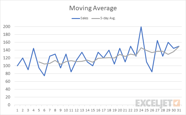
A moving average (also called a rolling average) is an average based on subsets of data at given intervals. Calculating an average at specific intervals smooths out the data by reducing the impact of random fluctuations. This makes it easier to see overall trends, especially in a chart. The larger the interval used to calculate a moving average, the more smoothing that occurs, since more data points are included in each calculated average.
Explanation
The formulas shown in the example all use the AVERAGE function with a relative reference set up for each specific interval. The 3-day moving average in E7 is calculated by feeding AVERAGE a range that includes the current day and the two previous days like this:
=AVERAGE(C5:C7) // 3-day average
The 5-day and 7-day averages are calculated in the same way. In each case, the range provided to AVERAGE is enlarged to include the required number of days:
=AVERAGE(C5:C9) // 5-day average
=AVERAGE(C5:C11) // 7-day average
All formulas use a relative reference for the range supplied to the AVERAGE function. As the formulas are copied down the column, the range changes at each row to include the values needed for each average.
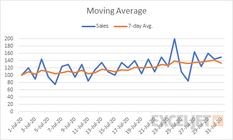
When the values are plotted in a line chart, the smoothing effect is clear:
Insufficient data
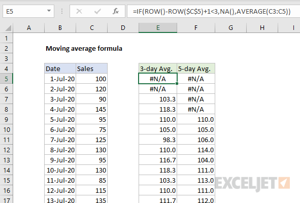
If you start the formulas in the first row of the table, the first few formulas won't have enough data to calculate a complete average, because the range will extend above the first row of data:
This may or may not be an issue, depending on the structure of the worksheet, and whether it's important that all averages are based on the same number of values. The AVERAGE function will automatically ignore text values and empty cells, so it will continue to calculate an average with fewer values. This is why it "works" in E5 and E6.
One way to clearly indicate insufficient data is to check the current row number and abort with #NA when there are less than n values. For example, for the 3-day average, you could use:
=IF(ROW()-ROW($C$5)+1<3,NA(),AVERAGE(C3:C5))
The first part of the formula simply generates a "normalized" row number, starting with 1:
ROW()-ROW($C$5)+1 // relative row number
In row 5, the result is 1, in row 6 the result is 2, and so on.
When the current row number is less than 3, the formula returns #N/A. Otherwise, the formula returns a moving average as before. This mimics the behavior of the Analysis Toolpak version of Moving Average, which outputs #N/A until the first complete period is reached.
However, as the number of periods increases, you will eventually run out of rows above the data and won't be able to enter the required range inside AVERAGE. For example, you can't set up a moving 7-day average with the worksheet as shown, since you can't enter a range that extends 6 rows above C5.
Variable periods with OFFSET
A more flexible way to calculate a moving average is with the OFFSET function. OFFSET can create a dynamic range, which means we can set up a formula where the number of periods is variable. The general form is:
=AVERAGE(OFFSET(A1,0,0,-n,1))
where n is the number of periods to include in each average. As above, OFFSET returns a range that is passed into the AVERAGE function. Below you can see this formula in action, where n is the named range E2. Starting at cell C5, OFFSET constructs a range that extends back to previous rows. This is accomplished by using a height equal to negative n. When E5 is changed to another number, the moving average recalculates on all rows:
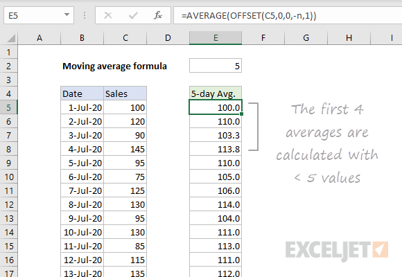
The formula in E5, copied down, is:
=AVERAGE(OFFSET(C5,0,0,-n,1))
Like the original formula above, the version with OFFSET will also have the problem of insufficient data in the first few rows, depending on how many periods are given in E5.
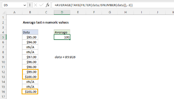
In the example shown, the averages calculate successfully because the AVERAGE function automatically ignores text values and blank cells, and there are no other numeric values above C5. So, while the range passed into AVERAGE in E5 is C1:C5, there is only one value to average, 100. However, as periods increase, OFFSET will continue to create a range that extends above the start of the data, eventually running into the top of the worksheet and returning a #REF error.
One solution is to "cap" the size of the range to the number of data points available. This can be done by using the MIN function to restrict the number used for height as seen below:
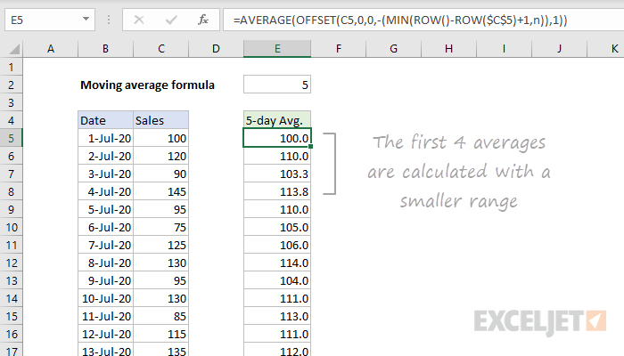
=AVERAGE(OFFSET(C5,0,0,-(MIN(ROW()-ROW($C$5)+1,n)),1))
This looks pretty scary but is actually quite simple. We are limiting the height passed into OFFSET with the MIN function:
MIN(ROW()-ROW($C$5)+1,n)
Inside MIN, the first value is a relative row number, calculated with:
ROW()-ROW($C$5)+1 // relative row number..1,2,3, etc.
The second value given to MIN is the number of periods, n. When the relative row number is less than n, MIN returns the current row number to OFFSET for height. When the row number is greater than n, MIN returns n. In other words, MIN simply returns the smaller of the two values.
A nice feature of the OFFSET option is that n can be easily changed. If we change n to 7 and plot the results, we get a chart like this:
Note: A quirk with the OFFSET formulas above is that they won't work in Google Sheets, because the OFFSET function in Sheets won't allow a negative value for height or width. The attached spreadsheet has workaround formulas for Google Sheets.