Summary
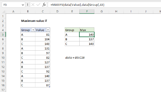
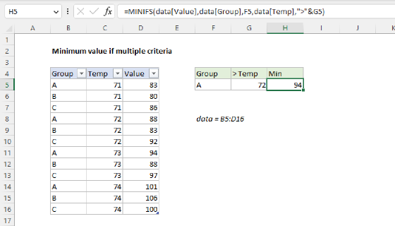
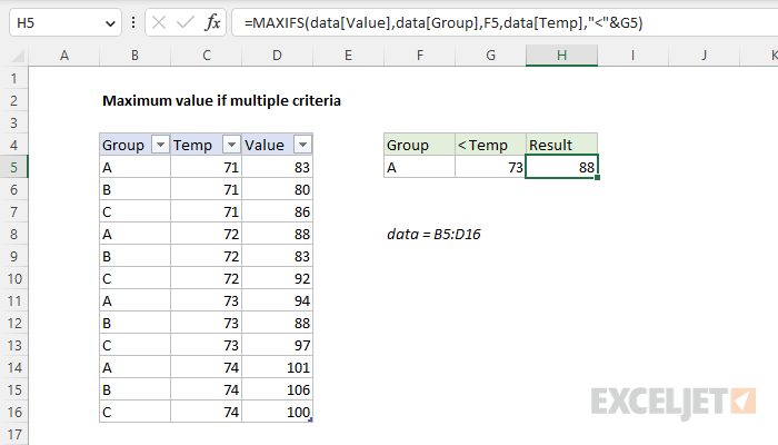
To get the maximum value in a set of data that meets multiple criteria, you can use a formula based on the MAXIFS function. In the example shown, the formula in H5 is:
=MAXIFS(data[Value],data[Group],F5,data[Temp],"<"&G5)
With "A" in cell F5 and the number 73 in cell G5, the result is 88. This is the maximum value in group "A" below a temperature of 73.
Generic formula
=MAXIFS(data,range1,criteria1,range2,criteria2)
Explanation
In this example, the goal is to get the maximum value for a given group below a specific temperature. In other words, we want the max value after applying multiple criteria. The easiest way to solve this problem is with the MAXIFS function. However, if you need more flexibility (i.e., you need to work with arrays and not ranges), you can use the MAX function with the FILTER function. In older versions of Excel without MAXIFS or FILTER, you can use a traditional array formula based on the MAX function and the IF function. Each approach is explained below.
Excel Table
For convenience, all data is in an Excel Table named data in the range B5:D16. Excel Tables are a convenient way to work with data in Excel because they (1) automatically expand to include new data and (2) offer structured references, which allow you to refer to data by name instead of by address. If you are new to Excel Tables, this article provides an overview.
Video: How to create an Excel Table
MAXIFS function
One way to solve this problem is with the MAXIFS function, which can get the maximum value in a range based on one or more criteria. The generic syntax for MAXIFS with two conditions looks like this:
=MAXIFS(max_range,range1,criteria1,range2,criteria2)
Note that each condition is defined by two arguments: range1 and criteria1 define the first condition, and range2 and criteria2 define the second condition. All conditions must be true in order for the value to be considered. We start off with the max_range, which is the Value column in the table:
=MAXIFS(data[Value],
Next, we add criteria to test for the group value entered in cell F5:
=MAXIFS(data[Value],data[Group],F5
If we enter the formula above as-is, we will get the maximum value in group "A". Next, we need to add a second condition to further restrict values below the temperature entered in cell G5:
=MAXIFS(data[Value],data[Group],F5,data[Temp],"<"&G5)
Notice we need to concatenate the less than operator ("<") to cell F5. This is a requirement of the MAXIFS function, which uses an unusual formula syntax shared by SUMIFS, COUNTIFS, etc. When we enter this formula, it returns the maximum value in group "A" below a temperature of 73. For reference, the same formula with conditions hardcoded looks like this:
=MAXIFS(data[Value],data[Group],"A",data[Temp],"<73")
MAXIFS will automatically ignore empty cells that meet the criteria. In other words, MAXIFS will not treat empty cells that meet the criteria as zero. On the other hand, MAXIFS will return zero (0) if no cells match the given criteria.
The MAXIFS function works well, but it does have one significant limitation: the range arguments inside MAXIFS must be actual ranges, you can't substitute arrays. If you need to use arrays, see the MAX + FILTER option below.
MAX + FILTER
In the dynamic array version of Excel, another way to solve this problem is with MAX and FILTER, like this:
=MAX(FILTER(data[Value],(data[Group]=F5)*(data[Temp]<G5)))
Inside the MAX function, the FILTER function is configured to filter values by group and temperature:
FILTER(data[Value],(data[Group]=F5)*(data[Temp]<G5))
Array is provided as the Value column in the table. The include argument is a simple expression:
(data[Group]=F5)*(data[Temp]<G5)
This is an example of using Boolean logic in Excel. Because there are 12 values in the table, each expression above generates an array of 12 TRUE and FALSE values like this:
{TRUE;FALSE;FALSE;TRUE;FALSE;FALSE;TRUE;FALSE;FALSE;TRUE;FALSE;FALSE}*{TRUE;TRUE;TRUE;TRUE;TRUE;TRUE;FALSE;FALSE;FALSE;FALSE;FALSE;FALSE}
The math operation of multiplication (*) converts the TRUE and FALSE values to 1s and 0s:
{1;0;0;1;0;0;1;0;0;1;0;0}*{1;1;1;1;1;1;0;0;0;0;0;0}
And the result is a single array as the include argument, like this:
FILTER(data[Value],{1;0;0;1;0;0;0;0;0;0;0;0})
Note that the 1s in this array correspond to values that are in group "A" with a temperature below 73. FILTER returns the two values that meet these criteria directly to the MAX function:
=MAX({83;88})
And MAX returns 88 as a final result. The primary advantage of using the MAX function with the FILTER function is that you don't need to provide a range of values on the worksheet. You can instead provide an array of values created with another operation. This is important when source data needs to be manipulated before a max value is calculated.
MAX + IF
In older versions of Excel that do not have the MAXIFS function or the FILTER function, you can solve this problem with an array formula based on the MAX function and the IF function, like this:
=MAX(IF((data[Group]=F5)*(data[Temp]<G5),data[Value]))
Note: This is an array formula and must be entered with control + shift + enter in Legacy Excel.
Working from the inside out, the IF function is evaluated first. The logical test inside IF is exactly the same as the logic explained above for FILTER:
(data[Group]=F5)*(data[Temp]<G5) // logical test
After the logic is evaluated, we have an array of 1s and 0s like this:
=MAX(IF({1;0;0;1;0;0;0;0;0;0;0;0},data[Value]))
The 1s correspond to rows where the group is "A" and the temperature is less than 73. The final result from IF is an array like this:
{83;FALSE;FALSE;88;FALSE;FALSE;FALSE;FALSE;FALSE;FALSE;FALSE;FALSE}
Looking at the values in this array, you can see that the IF function acts like a filter: only values associated with group "A" and a temperature less than 73 make it through the filter. The other values are replaced with FALSE. The IF function delivers this array directly to the MAX function:
=MAX({83;FALSE;FALSE;88;FALSE;FALSE;FALSE;FALSE;FALSE;FALSE;FALSE;FALSE})
The MAX function automatically ignores FALSE values and returns the maximum number in the array: 88.
Alternative syntax with nested IFs
The array formula above uses Boolean logic to streamline the formula, but another option you might run into is nesting one IF formula inside another, like this:
=MAX(IF(data[Group]=F5,IF(data[Temp]<G5,data[Value])))
Note: This is an array formula and must be entered with control + shift + enter in Legacy Excel.
Each IF formula applies a separate condition, so the values are filtered in two steps instead of one. This works fine, but the formula gets more complicated as additional criteria are added, since each condition requires another IF function. The advantage Boolean logic version of the formula is that you can add additional criteria without adding more IF functions.