Max value on given weekday

In this example, the goal is to calculate the maximum value that occurs in a set of data on a given weekday (i.e. Monday, Tuesday, Wednesday, Thursday, Friday). In the current version of Excel, the simplest approach is to use the FILTER function. In older versions of Excel, you can use a traditional array formula based on the MAX function with the IF function. Both approaches are explained below.

FILTER function

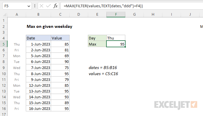
The most straightforward way to solve this problem is with the FILTER function, the MAX function, and the TEXT function. In the example shown, the formula in cell F5 is:

=MAX(FILTER(values,TEXT(dates,"ddd")=F4))

Working from the inside out, the TEXT function is configured to compare the "day" for each date, abbreviated to three letters, with the day value in cell F4:

TEXT(dates,"ddd")=F4)

Here, the TEXT function is using the custom number format "mmm" to calculate day abbreviations for the dates. Because there are 12 dates in dates (B5:B16) the TEXT function returns an array of 12 day abbreviations like this:

{"Thu";"Fri";"Mon";"Tue";"Wed";"Thu";"Fri";"Mon";"Tue";"Wed";"Thu";"Fri"}=F4

When this array is compared to cell F4, the result is an array that contains 12 TRUE and FALSE values:

{TRUE;FALSE;FALSE;FALSE;FALSE;TRUE;FALSE;FALSE;FALSE;FALSE;TRUE;FALSE}

In this array, the TRUE values correspond to dates that are Thursdays in the data. This array is returned directly to the FILTER function as the include argument with the named range values (C5:C16) as the array argument. FILTER uses the array to "filter" the values and returns the three values that occur on Thursdays directly to the MAX function:

=MAX({85;95;89})

MAX then returns 95 as a final result. If the value in F4 is changed to another day, the formula calculates a new result.

Legacy Excel

In older versions of Excel without the FILTER function, you can use a traditional array formula based on the MAX function and the IF function:

=MAX(IF(TEXT(dates,"ddd")=F4,values))

Note: this is an array formula and must be entered with control + shift + enter in Legacy Excel.

Working from the inside out, the TEXT function is used to extract a weekday value for each date:

=TEXT(dates,"ddd")

The text string "ddd" is a number format for abbreviated day names. Because there are 12 dates in B5:B16, the result is an array with 12 abbreviated day names, which is then compared to cell F4:

{"Thu";"Fri";"Mon";"Tue";"Wed";"Thu";"Fri";"Mon";"Tue";"Wed";"Thu";"Fri"}=F4

With "Thu" in F4, this operation results in another array that contains only TRUE and FALSE values:

{TRUE;FALSE;FALSE;FALSE;FALSE;TRUE;FALSE;FALSE;FALSE;FALSE;TRUE;FALSE}

Note each TRUE corresponds to a Thursday. This array is returned to the IF function as the logical_test. IF then acts as a filter to screen out values on other days of the week. The final result from IF, which is returned directly to the MAX function, looks like this:

=MAX({85;FALSE;FALSE;FALSE;FALSE;95;FALSE;FALSE;FALSE;FALSE;85;FALSE})

Note the only values that survive the trip through IF are those associated with Thursdays, the other values are now FALSE. MAX automatically ignores FALSE values and returns the highest remaining value, 95.

With AGGREGATE

For a more geeky formula that doesn't require control + shift + enter in Legacy Excel, you can use the AGGREGATE function like this:

=AGGREGATE(14,6,values/(TEXT(dates,"ddd")=F4),1)

Here we give AGGREGATE 14 for the function argument (LARGE) and 6 for option argument (ignore errors). Then we build a logical expression using the TEXT function to check all dates for Thursdays. The result of this operation is is an array of TRUE/FALSE values, which become the denominator of the original values. When used in a math operation, FALSE evaluates as zero, and throws a #DIV/0! error. TRUE evaluates as 1 and returns the original value. The final array of values and errors acts like a filter. AGGREGATE ignores all errors and returns the largest (maximum) of the surviving values.

Note: The reason this formula works in older versions of Excel without being entered as an array formula is that AGGREGATE, like the SUMPRODUCT function, can handle many array operations natively. In the future this use of AGGREGATE will diminish since the new dynamic array engine in Excel makes these kind of workarounds unnecessary.

MAXIFS function

You might wonder why we aren't using the MAXIFS function, which can calculate a maximum value based on one or more criteria. The problem is that MAXIFS is a ranged-based function, and won't accept an array from another function like TEXT. If you want to use MAXIFS, you could add a helper column to the data that calculates weekday abbreviations with TEXT, then use MAXIFS with the helper column as the criteria range.