Summary
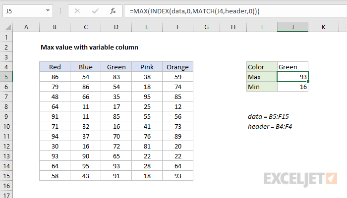
To retrieve the max value in a set of data, where the column is variable, you can use INDEX and MATCH together with the MAX function. In the example shown the formula in J5 is:
=MAX(INDEX(data,0,MATCH(J4,header,0)))
where data (B5:F15) and header (B4:F4) are named ranges.
Generic formula
=MAX(INDEX(data,0,MATCH(column,header,0)))
Explanation
Note: If you are new to INDEX and MATCH, see: How to use INDEX and MATCH
In a standard configuration, the INDEX function retrieves a value at a given row and column. For example, to get the value at row 2 and column 3 in a given range:
=INDEX(range,2,3) // get value at row 2, column 3
However, INDEX has a special trick – the ability to retrieve entire columns and rows. The syntax involves supplying zero for the "other" argument. If you want an entire column, you supply row as zero. If you want an entire row, you supply column as zero:
=INDEX(data,0,n) // retrieve column n
=INDEX(data,n,0) // retrieve row n
In the example shown, we want to find the maximum value in a given column. The twist is that the column needs to be variable so it can be easily changed. In F5, the formula is:
=MAX(INDEX(data,0,MATCH(J4,header,0)))
Working from the inside out, we first use the MATCH function to get the "index" of the column requested in cell J4:
MATCH(J4,header,0) // get column index
With "Green" in J4, the MATCH function returns 3, since Green is the third value in the named range header. After MATCH returns a result, the formula can be simplified to this:
=MAX(INDEX(data,0,3))
With zero provided as the row_number, INDEX returns all values in column 3 of the named range data. The result is returned to the MAX function in an array like this:
=MAX({83;54;35;17;85;16;70;72;65;93;91})
And MAX returns the final result, 93.
Minimum value
To get the minimum value with a variable column, you can simply replace the MAX function with the MIN function. The formula in J6 is:
=MIN(INDEX(data,0,MATCH(J4,header,0)))
With FILTER
The new FILTER function can also be used to solve this problem, since FILTER can filter data by row or by column. The trick is to construct a logical filter that will exclude other columns. COUNTIF works well in this case, but it must be configured "backwards", with J4 as the range, and header for criteria:
=MAX(FILTER(data,COUNTIF(J4,header)))
After COUNTIF runs, we have:
=MAX(FILTER(data,{0,0,1,0,0}))
And FILTER delivers the 3rd column to MAX, same as the INDEX function above.
As an alternative to COUNTIF, you can use ISNUMBER + MATCH instead:
=MAX(FILTER(data,ISNUMBER(MATCH(header,J4,0))))
The MATCH function is again set up "backwards", so that we get an array with 5 values that will serve as the logical filter. After ISNUMBER and MATCH run, we have:
=MAX(FILTER(data,{FALSE,FALSE,TRUE,FALSE,FALSE}))
And FILTER again delivers the 3rd column to MAX.