Explanation
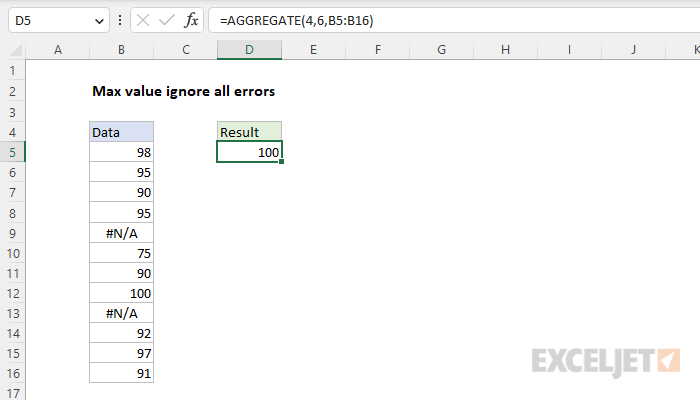
In this example, the goal is to return the maximum value in a set of data while ignoring any errors that might exist. This problem can be solved with the AGGREGATE function or with the MAXIFS function, as explained below.
MAX with errors
The standard way to retrieve the maximum value in a range of data is the MAX function. However, if we try to use MAX like this:
=MAX(B5:B16) // returns #N/A
The MAX function returns #N/A as a result because the range B5:B16 contains errors. The problem with MAX is that it will return an error if the data contains errors.
AGGREGATE function
The AGGREGATE function is a useful function that can run an aggregate calculation like AVERAGE, COUNT, MAX, MIN, etc., while optionally ignoring errors. A total of 19 operations are available, specified by a function number provided as the first argument. The table here contains a complete list of available operations. In this case we want to use the number 4 for function_num, which specifies the MAX operation. For the second argument, options, we provide the number 6, which indicates "ignore all errors". For array, we provide the range B5:B16. The final formula looks like this:
=AGGREGATE(4,6,B5:B16)
To recap, the number 4 specifies MAX, and the number 6 is an option to ignore errors. With these settings, AGGREGATE returns the maximum value in the range, which is 100.
Alternative with MAXIFS
Another way to solve this problem is with the MAXIFS function, which can calculate a max value after applying one or more conditions to filter out unwanted values. If values in the data set are known to be positive, a simple way to ignore errors is to check for values greater than zero like this:
=MAXIFS(data,data,">0")
This works because the "greater or equal to zero" expression effectively removes error values, and MAXIFS returns the maximum value from the remaining 10 values, 100. You can also use the MAXIFS function with more specific criteria like this:
=MAXIFS(data,data,"<>#N/A") // ignore NA errors
=MAXIFS(data,data,"<>#DIV/0!") // ignore DIV/0 errors
=MAXIFS(data,data,"<>#N/A",data,"<>#DIV/0!") // ignore both
All formulas above use the not equal to ("<>") operator. The first formula calculates a maximum after excluding #N/A errors. The second formula calculates a maximum after excluding #DIV/0! errors. The last formula uses two conditions to exclude both #N/A and #DIV/0! errors.


