List holidays between two dates

To list holidays that occur between two dates, you can use a formula based on the TEXTJOIN and IF functions.

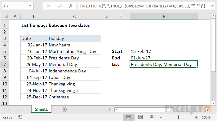
In the example shown, the formula in F8 is:

{=TEXTJOIN(", ",TRUE,IF(B4:B12>=F5,IF(B4:B12<=F6,C4:C12,""),""))}

This is an array formula and must be entered with control + shift + enter.

Explanation

At a high level, this formula uses a nested IF function to return an array of holidays between two dates. This array is then processed by the TEXTJOIN function, which converts the array to text using a comma as the delimiter.

Working from the inside out, we generate the array of matching holidays using a nested IF:

IF(B4:B12>=F5,IF(B4:B12<=F6,C4:C12,""),"")

If the dates in B4:B12 are greater than or equal the start date in F5, and if the dates in B4:B12 are less than or equal the end date in F6, then IF returns a an array of holidays. In the example shown, the list looks like this:

{"";"";"Presidents Day";"Memorial Day";"";"";"";"";""}

This array is then delivered to the TEXTJOIN function as the text1 argument, where the delimiter is set to ", " and ignore_empty is TRUE. The TEXT JOIN function processes the items in the array and returns a string where every non-empty item is separated by a comma plus space.

Note: the TEXTJOIN function is a new function available in Office 365 and Excel 2019.