Summary
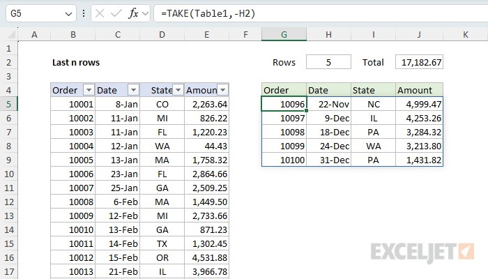
To get the last n rows from a range or table, you can use a formula based on the TAKE function. In the example shown, the formula in cell G5 is:
=TAKE(Table1,-H2)
Where the value in cell H2 is the number of rows to retrieve from the bottom of an Excel Table named Table1. This formula is dynamic and will update automatically as the number of rows in the table changes, or when the number of rows to retrieve in H2 is changed.
Generic formula
=TAKE(range,-n)
Explanation
When you are working with a large table that extends beyond the visible area of a worksheet, you might want to see the most recent data in the table without scrolling to the bottom of the table. Examples of this kind of data include things like:
- Recent deposits or expenses
- Recent transactions
- Recent stock prices
- Recent orders
- Recent invoices
In this example, the goal is to dynamically retrieve the last n rows of a table or range, so that you can quickly check the entries at the bottom, where n is a value that can be easily changed. The main challenge of this problem is that you don't know where the table ends, so the formula needs to work this out. This is a great use case for the TAKE function.
Table of Contents
- Note on Excel Tables
- The TAKE function
- TAKE to get the last n rows
- Calculating a total amount
- Sorting the last n rows in reverse order
- Sorting the last n rows in reverse order with a checkbox
- Legacy Excel Formulas
- Multi-cell array formula to get the last n rows
- Flagging last n rows in a range
- Flagging last n rows in a table
Note on Excel Tables
This example uses Excel Tables to store the data we are working with, because Excel Tables automatically expand to fit the data as it grows. In other words, they are an easy way to create a dynamic range in Excel. One consequence of using tables is that each table needs a unique name. As a result, the examples below are named Table1, Table2, Table3, and Table4 on each of the four sheets. The data in each table is the same; only the names are different.
If you don't want to use an Excel Table, you could use the TRIMRANGE function or the new dot operator to create your own dynamic range.
The TAKE function
The Excel TAKE function returns a subset of a given array. The number of rows and columns to return is provided by separate rows and columns arguments.
=TAKE(array,rows,columns)
Where rows is the number of rows to return and columns is the number of columns to return. When positive numbers are provided for rows and columns, TAKE returns values from the start of the array, starting at the upper left cell. For example, to get the first cell in a range, you can use:
=TAKE(range,1,1) // returns the first cell in the range
When negative numbers are provided for rows and columns, TAKE returns values from the end of the array, starting at the lower right cell. For example, to get the last cell in a range, you can use:
=TAKE(range,-1,-1) // returns the last cell in the range.
You can use the same approach to retrieve whole rows:
=TAKE(range,1) // returns the first row in the range
=TAKE(range,-1) // returns the last row in the range
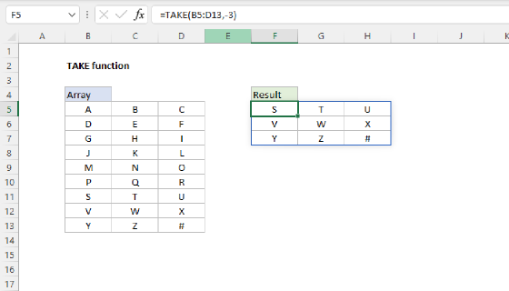
TAKE to get the last n rows
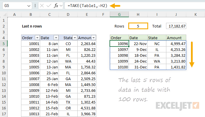
Moving back to the worksheet shown, we can easily use TAKE to get the last 5 rows in the table shown with a formula like this in cell G5:
=TAKE(Table1,-5)
To make the formula more dynamic, so that it will automatically respond to a number of rows typed in cell H2, we simply need to replace the hard-coded 5 with a reference to cell H2:
=TAKE(Table1,-H2)
You can see how this works in the worksheet below. In the first screen, we have 5 in H2, so the formula returns the last 5 rows in the table.
In the next screen, we have entered 10 in H2, so the formula returns the last 10 rows in the table:
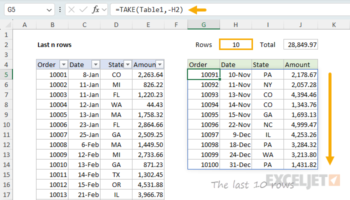
Notice we need to negate the value in H2 (-H2) in order to pull rows from the end of the table.
Calculating a total amount
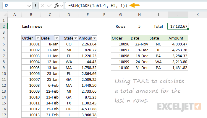
To calculate a total amount from the last n rows, we can use a formula like this in cell J2:
=SUM(TAKE(Table1,-H2,-1))
This formula uses the TAKE function to get the last 5 rows of the last column in the table (Amount), then feeds those values into the SUM function, which returns a total:
Another option is to reference the Amount column directly using a structured reference like this:
=SUM(TAKE(Table1[Amount],-H2))
Both formulas will return a dynamic total for the last n rows in the table, based on the value in cell H2.
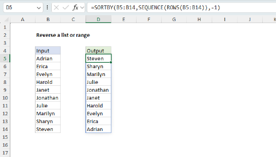
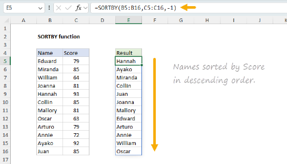
Sorting the last n rows in reverse order
If you want to sort the last n rows in "reverse order" so that the last row is displayed first, you can use a formula like this:
=SORTBY(TAKE(Table2,-H2),SEQUENCE(H2),-1)
This formula will return the last n rows in the table sorted in reverse order by position, so that the last row is displayed first. You can see how this works in the worksheet below:
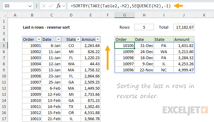
The SEQUENCE function is used to create a sequence of numbers from 1 to n, which is then used to sort the rows in reverse order. For details on how this formula works, see Reversing a list or range.
Sorting the last n rows in reverse order with a checkbox
One interesting option we can add to the formula above is the ability to sort the last n rows in reverse order conditionally, using a checkbox to control the sort order. In the worksheet below, we have made the reverse sort optional by inserting a checkbox to cell J2 and using a formula like this in cell G5:
=LET(rows,TAKE(Table3,-H2),IF(J2,SORTBY(rows,SEQUENCE(H2),-1),rows))
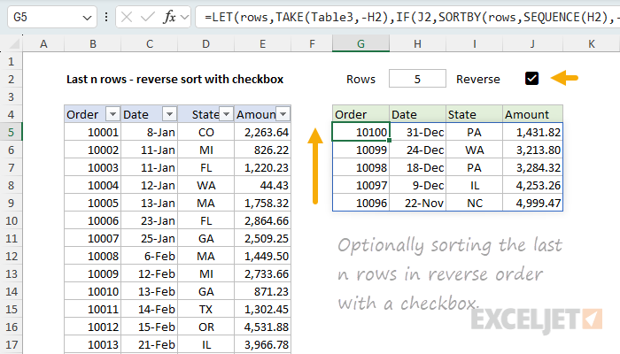
This formula uses the LET function to create a variable called rows, which becomes the n rows of the table using the original formula above. Next, the IF function is used to conditionally sort the rows in reverse order based on the state of the checkbox in cell J2. If the checkbox in cell J2 is checked (TRUE), we sort the rows in reverse order using the SORTBY function:
=SORTBY(rows,SEQUENCE(H2),-1)
If the checkbox in cell J2 is unchecked (FALSE), the IF function returns rows as is. The result is a dynamic list of the last n rows in the table, sorted in reverse order when the checkbox is checked, and in the original order when the checkbox is unchecked.
Note: You could use a simpler formula based on the SORT function to sort in reverse order by any column in the table that will work for a "reverse" sort. The advantage of using SORTBY + SEQUENCE is that it will work even for tables that do not contain a numeric column to sort by.
Legacy Excel Formulas
This section contains some formulas that are useful in older versions of Excel that do not have new functions like TAKE and SEQUENCE, and do not support dynamic arrays. These formulas are not as efficient as the ones using the new functions, but they are still useful in some cases.
Multi-cell array formula to get the last n rows
One way to get the last n rows in an older version of Excel is to use a multi-cell array formula. Multi-cell array formulas are the precursor to dynamic arrays in Excel, and they work in a similar way. The trick with a multi-cell array formula is to select the entire range that represents the maximum size the formula needs to cover and then enter the same formula using Ctrl+Shift+Enter in the entire range. For example, with the worksheet we've been working with above, first select the range G5:J29 (25 rows) and enter the following formula in cell G5, then press Ctrl+Shift+Enter to enter the formula as an array formula:
{=IF(ROW()-ROW(G5)+1<=H2,INDEX(Table4,ROWS(Table4)-(H2-1),0):INDEX(Table4,ROWS(Table4),0),"")}
Note: There is no need to copy this formula down and across because it is entered in all cells at the same time. You will see the curly braces around the entire formula in the formula bar when the formula is entered with Ctrl+Shift+Enter. These braces are not part of the formula itself. They are simply an indication that the formula was entered as an array formula. They will disappear when you edit the formula.
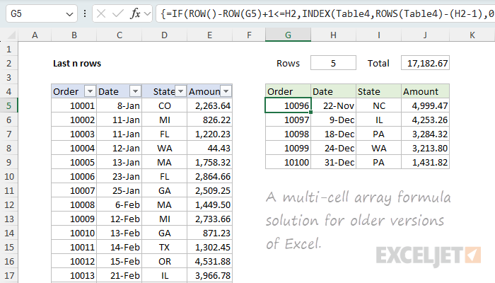
At a high level, the formula uses the IF function to check if the "current row" is one of the last n rows in the table, using the value for n in cell H2. If it is, the formula retrieves the rows from the table using the INDEX function. If the current row is greater than n, the formula returns an empty string. The row check snippet looks like this:
=ROW()-ROW(G5)+1<=H2
The ROW function is used to get the row number of the current cell, and the row number of the first cell in the table (G5). The difference between the two plus 1 gives us the current row number in the output range. If this value is less than or equal to the number of rows to retrieve, the formula returns the last n rows in the table using the INDEX function:
=INDEX(Table4,ROWS(Table4)-(H2-1),0):INDEX(Table4,ROWS(Table4),0)
Notice the colon (:) between the two INDEX functions. This is a special operator that returns a range of cells. Essentially, we are building a range from the references created by the two INDEX functions. The INDEX on the right is a reference to the last row in the table, and the INDEX on the left is a reference to the first row in the table that we want to include in the output. When we join the two references with the colon, we get a range that contains the last n rows in the table.
Note: You could also use the OFFSET function to solve this problem. However, OFFSET is a volatile function and will recalculate every time the worksheet is recalculated, so I avoid using it when possible.
Flagging last n rows in a range
Sometimes you may want to flag the last n rows in a table or range, so that you can easily identify them. One way to do this is to use a helper column with a formula that returns TRUE if a row is a "last n row", and FALSE if not. For example, in the worksheet shown below, the formula in cell E5, copied down, is:
=ROW()-ROW(INDEX(data,1,1))+1>ROWS(data)-n
Where data (B5:E15) and n (G5) are named ranges. This formula returns TRUE if a row is a "last n row", and FALSE if not.
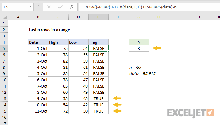
In brief, we get the current row in the workbook, then subtract the first row number of the range plus 1. The result is an adjusted row number that begins at 1. The INDEX function is simply a way to get the first cell in a given range:
ROW(INDEX(data,1,1) // first cell
This is for convenience only. The formula could be rewritten as:
=ROW()-ROW($E$5)+1
Once we have a current row number, we can compare the row number to the total rows in the data less n:
current_row > ROWS(data)-n
This expression returns TRUE if the current row is one of the last n rows we are looking for. Otherwise, it returns FALSE.
Flagging last n rows in a table
If data is in an Excel table, the formula above can be adapted like this:
=ROW()-@ROW(Table1)+1>ROWS(Table1)-n
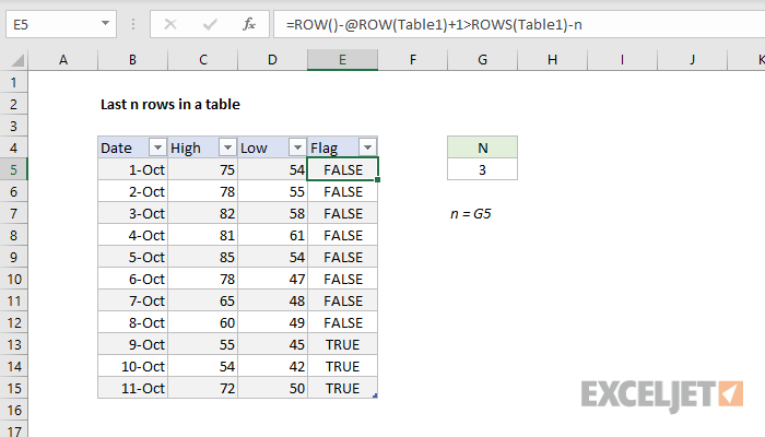
The logic is exactly the same as the previous formula, but we use a slightly different approach to get the first cell in the table:
@ROW(Table1)
The @ operator means implicit intersection. You can think of it as indicating "single":
=ROW(Table1) // returns {5;6;7;8;9;10;11;12;13;14;15}
=@ROW(Table1) // returns {5}
As before, the table formula returns TRUE in "last n rows" and FALSE in others.