Summary
The #N/A error usually appears when something can't be found or identified. However, #N/A errors can also be caused by extra space characters, misspellings, or an incomplete lookup table. The functions mostly commonly affected by the #N/A error are classic lookup functions, including VLOOKUP, HLOOKUP, LOOKUP, and MATCH. See below for more information and steps to resolve.
Generic formula
=IFERROR(FORMULA(),"message")
Explanation
About the #N/A error
The #N/A error appears when something can't be found or identified. It is often a useful error, because it tells you something important is missing – a product not yet available, an employee name misspelled, a color option that doesn't exist, etc.
However, #N/A errors can also be caused by extra space characters, misspellings, or an incomplete lookup table. The functions mostly commonly affected by the #N/A error are classic lookup functions, including VLOOKUP, HLOOKUP, LOOKUP, and MATCH.
The best way to prevent #N/A errors is to make sure lookup values and lookup tables are correct and complete. If you see an unexpected #N/A error, check the following first:
- The lookup value is spelled correctly and does not contain extra space characters.
- Values in the lookup table are spelled correctly and do not contain extra space.
- The lookup table is contains all required values.
- The lookup range provided to the function is complete (i.e. does not "clip" data).
- Lookup value type = lookup table type (i.e. both are text, both are numbers, etc.)
- Matching (approximate vs. exact) is set correctly.
Note: if you get an incorrect result, when you should see a #N/A error, make sure you have exact matching configured correctly. Approximate match mode will happily return all kinds of results that are totally incorrect :)
Trapping the #N/A error with IFERROR
One option for trapping the #N/A error is the IFERROR function. IFERROR can gracefully catch any error and return an alternative result .
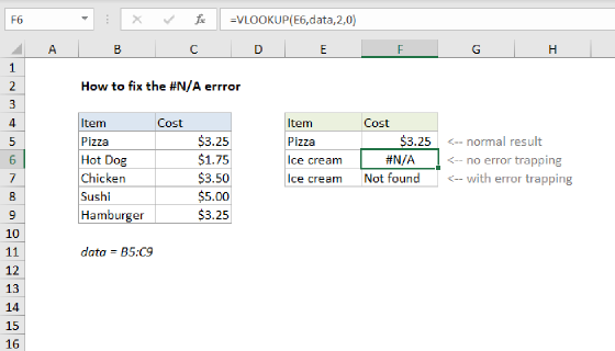
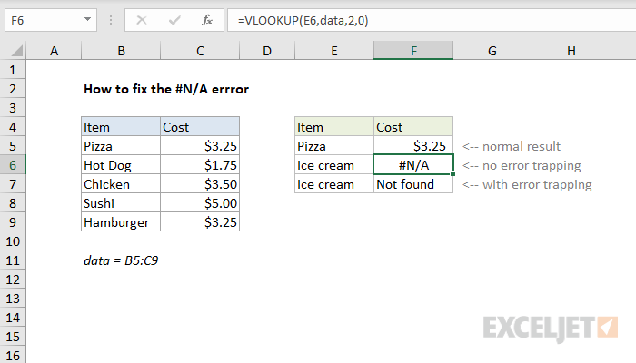
In the example shown, the #N/A error appears in cell F5 because "ice cream" does not exist in the lookup table, which is the named range "data" (B5:C9).
=VLOOKUP(E5,data,2,0) // "ice cream" is not found
To handle this error, the IFERROR function is wrapped around the VLOOKUP formula like this:
=IFERROR(VLOOKUP(E7,data,2,0),"Not found")
If the VLOOKUP function returns an error, the IFERROR function "catches" that error and returns "Not found".
Trapping the #N/A error with IFNA
The IFNA function can also trap and handle #N/A errors specifically. The usage syntax is the same as with IFERROR:
=IFERROR(VLOOKUP(A1,table,column,0),"Not found")
=IFNA(VLOOKUP(A1,table,column,0),"Not found")
The advantage of the IFNA function is that it is more surgical, targeting just #N/A errors. The IFERROR function, on the other hand, will catch any error. For example, even if you spell VLOOKUP incorrectly, IFERROR will return "Not found".
No message
If you don't want to display any message when you trap an #N/A error (i.e. you want to display a blank cell), you can use an empty string ("") like this:
=IFERROR(VLOOKUP(E7,data,2,0),"")
INDEX and MATCH
The MATCH function also returns #N/A when a value is not found. If you are using INDEX and MATCH together, you can trap the #N/A error in the same way. Based on the example above, the formula in F5 would be:
=IFERROR(INDEX(C5:C9,MATCH(E5,B5:B9,0)),"Not found")
Read more about INDEX and MATCH.
Forcing the #N/A error
If you want to force the #N/A error on a worksheet, you can use the NA function. For example, display #N/A in a cell when A1 equals zero, you can use a formula like this:
=IF(A1=0, NA())