Summary
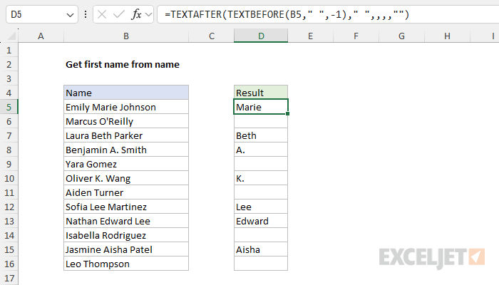
To extract the middle name from a full name, you can use a formula based on the TEXTAFTER and TEXTBEFORE functions like this:
=TEXTAFTER(TEXTBEFORE(B5," ",-1)," ",,,,"")
As the formula is copied down, it returns the middle name when present, and an empty string ("") when there is no middle name.
Note: As of this writing, TEXTBEFORE and TEXTAFTER are is only available in Excel 365. See below for an alternative formula that will work in older versions of Excel.
Generic formula
=TEXTAFTER(TEXTBEFORE(name," ",-1)," ",,,,"")
Explanation
In this example, the goal is to return the middle name from a full name in "First Middle Last" format. In the current version of Excel this is a fairly simple problem using the TEXTAFTER and TEXTBEFORE functions. In older versions of Excel, a similar formula is significantly more complicated, based on the MID function and multiple FIND functions. Both approaches are explained below.
Modern solution
In the latest version of Excel you can solve this problem with the TEXTAFTER and TEXTBEFORE functions like this:
=TEXTAFTER(TEXTBEFORE(B5," ",-1)," ",,,,"")
As the formula is copied down, it returns the middle name when present, and an empty string ("") when there is no middle name. Working from the inside out, the TEXTBEFORE function is first used to extract all text that occurs after the last space in the name:
TEXTBEFORE(B5," ",-1) // returns "Emily Marie"
- text - the full name in cell B5
- delimiter - a single space (" ")
- instance_num - provided as -1 (first space from the end)
The trick here is using -1 for instance_num. A positive instance number tells TEXTBEFORE to count from the start of the text string. A negative instance number tells TEXTBEFORE to count from the end. The result is "Emily Marie" (the name without the last name) which is delivered to the TEXTAFTER function:
=TEXTAFTER("Emily Marie"," ",,,,"")
- text - result from TEXTBEFORE
- delimiter - a single space (" ")
- instance_num - omitted, defaults to 1
- match_mode - omitted
- match_end - omitted
- if_not_found - an empty string ("")
Essentially, we are asking TEXTAFTER for the text after the (first) space. Importantly, we also provide an empty string ("") for the if_not_found argument to gracefully handle cases where there is no middle name.
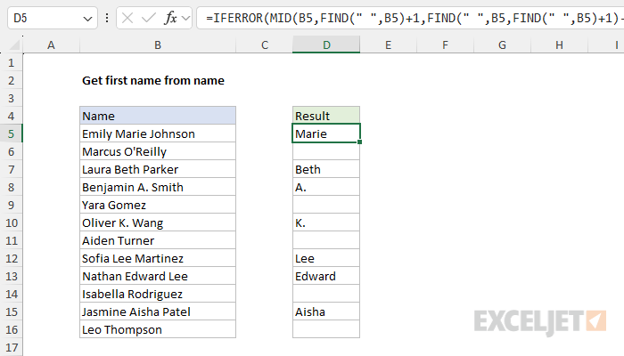
Legacy solution
In older versions of Excel that do not provide the TEXTAFTER or TEXTBEFORE functions, it is possible to use a more complex formula to extract the middle name:
=MID(B9,FIND(" ",B9)+1,FIND(" ",B9,FIND(" ",B9)+1)-FIND(" ",B9)-1)
This Excel formula is designed to extract the text between the first and second space characters in the cell B5. At a high level, we are using the MID function to extract a substring from the text in cell B5, where the start_num is the position to start the extraction, and num_chars is the number of characters to extract:
MID(B5,start_num,num_chars)
The challenge is in working out the correct values for start_num and num_chars. To calculate a start number, we use the FIND function like this:
FIND(" ",B5)+1 // start_num
This finds the position of the first space in B5 and adds 1. This calculation is used to set the start_num for the MID function, effectively starting the extraction from the character immediately after the first space. Next, we need to calculate the number of characters to extract. This is a more difficult problem. First, we find the position of the second space in B5 like this:
FIND(" ",B5,FIND(" ",B5)+1)
Here, we take advantage of the fact that the FIND function has as optional third argument called start_num, which controls where FIND begins its search. When no value is provided, start_num will default to 1 and FIND will begin searching from the beginning of the text string. To find the second space, we are asking FIND to begin searching one character after the first space:
FIND(" ",B5)+1 // one char after first space
Once we know the location of the second space, we need to subtract the location of the first space:
FIND(" ",B5,FIND(" ",B5)+ )-FIND(" ",B5)-1
This code calculates the number of characters between the first and second space by subtracting the position of the first space from the position of the second space and then subtracting 1. The result is delivered to the MID function as the num_chars argument, and MID then extracts all text between the two spaces.
=MID(B5,FIND(" ",B5)+1,FIND(" ",B5,FIND(" ",B5)+1)-FIND(" ",B5)-1)
=MID(B5,7,FIND(" ",B5,FIND(" ",B5)+1)-FIND(" ",B5)-1)
=MID(B5,7,FIND(" ",B5,FIND(" ",B5)+1)-FIND(" ",B5)-1)
=MID(B5,7,FIND(" ",B5,6+1)-6-1)
=MID(B5,7,FIND(" ",B5,7)-6-1)
=MID(B5,7,12-6-1)
=MID(B5,7,5)
="Marie"
The formula above will work correctly when there are two spaces in the name. However, when a second space is not found (i.e. there is no middle name, FIND will return a #VALUE! error. An easy way to manage this error is to embed the original formula into the IFERROR function:
=IFERROR(MID(B5,FIND(" ",B5)+1,FIND(" ",B5,FIND(" ",B5)+1)-FIND(" ",B5)-1),"")
Now when a second space is not found, FIND will return a #VALUE! error, and IFERROR will catch that error and return an empty string (""), which looks like a blank cell in Excel.