Summary
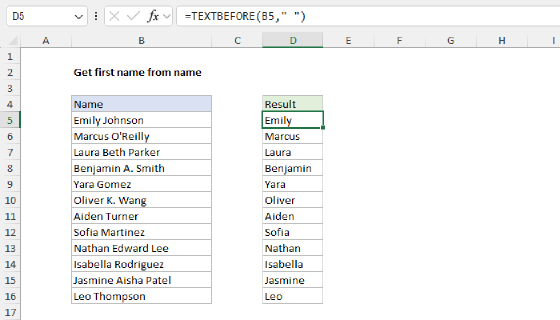
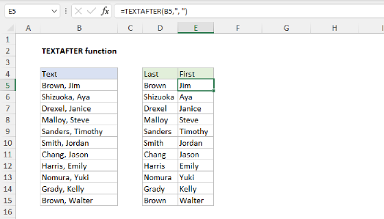
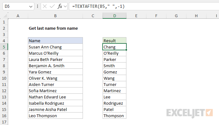
To extract the last name from a full name in <first> <middle> <last> format, you can use the TEXTAFTER function. In the worksheet shown, the formula in cell D5 is:
=TEXTAFTER(B5," ",-1)
As the formula is copied down, it returns the lat name from each name listed in column B, ignoring middle names when they exist.
Note: As of this writing, the TEXTAFTER function is only available in Excel 365. See below for an alternative formula that will work in older versions of Excel.
Generic formula
=TEXTAFTER(A1," ",-1)
Explanation
In this example, the goal is to extract the last name from names that appear in <first> <middle> <last> format, where the middle name is not always present. The easiest way to do this is with the newer TEXTAFTER function. In older versions of Excel, you can use a significantly more complex formula based on the RIGHT, FIND, and SUBSTITUTE functions. Both options are explained below.
Note: This is a great example of how new functions in Excel like TEXTBEFORE and TEXTAFTER are game-changers that can radically simplify formulas. Note the contrast between the modern solution and the legacy solution.
Modern solution
In the current version of Excel, the TEXTAFTER function is the best way to solve this problem. TEXTAFTER extracts text that occurs after a given delimiter. In its simplest form, TEXTAFTER only requires two arguments, text and delimiter. However, in this case, we also need to provide an instance number:
=TEXTAFTER(text,delimiter,instance_num)
In the worksheet shown, the formula we are using to return the last name looks like this:
=TEXTAFTER(B5," ",-1)
- text - B5, the full name in column B
- delimiter - " ", a single space
- instance_num - provided as -1, the first space from the end
The key here is setting instance_num to -1. Normally, a positive instance number tells TEXTAFTER to count instances from the left. A negative instance number tells TEXTAFTER to count instances from the right. In other words, we are asking TEXTAFTER for the text after the last space. This is important, because some names have middle names, and we need to ignore the first space in that case. TEXTAFTER has many other options that you can read more about here.
Legacy solution
In older versions of Excel that do not offer the TEXTAFTER function, you can use an alternative formula that looks like this:
=MID(B5,FIND("*",SUBSTITUTE(B5," ","*",LEN(B5)-LEN(SUBSTITUTE(B5," ",""))))+1,100)
Note: it is also possible to use the RIGHT function in a similar formula, but using MID is a bit of a shortcut.
This is a complicated formula. One reason it's complicated is that we don't have a direct way to find the last space in a name, which is important when a name contains more than two words (i.e. contains one or more middle names). As a result, we need to employ some trickery with the SUBSTITUTE function to locate and mark the last space in the name with an asterisk (*).
At the core, this formula uses the MID function to extract characters in the name starting at a particular location. The complex part of the formula does just one thing: it calculates how many characters need to be extracted, represented by n below:
=MID(B5,n,100)
The code that calculates n is below:
FIND("*",SUBSTITUTE(B5," ","*",LEN(B5)-LEN(SUBSTITUTE(B5," ",""))))+1
At a high level, the snippet above replaces the last space (" ") in the full name with an asterisk () and then uses the FIND function to determine the numeric position of the asterisk (). Once we have that number, we simply add 1 to determine a start_num for MID.
How does the code replace only the last space with an asterisk? This is the clever part. Buckle up, because the explanation gets a bit technical. The key to this formula is this bit:
SUBSTITUTE(B5," ","*",LEN(B5)-LEN(SUBSTITUTE(B5," ","")))
Normally, the SUBSTITUTE function will replace all instances of old_text with new_text. However, SUBSTITUTE has an optional fourth argument called instance_num that specifies which "instance" of the old text should be replaced. If the argument is omitted, all instances are replaced. If a number like 2 is provided, SUBSTITUTE will replace only the second instance.
At this point, the problem becomes how to calculate the correct instance_num. Looking back at the names in column B, we can see that we want to provide instance number as 2 when a name contains a middle name, and instance number as 1 when there is a middle name. The way we solve the problem is to count the number of spaces in the name, which we do in the snippet below:
LEN(B4)-LEN(SUBSTITUTE(B4," ",""))
This is a fairly common pattern in Excel formulas that must calculate how many times a character appears in a text string. In brief, we calculate the total length of the text string with the LEN function, then subtract the length of the text string after the target character has been removed with SUBSTITUTE. You can find a more detailed explanation here.
In cell B5, the name is "Susan Ann Chang", so the code above evaluates like this:
=LEN(B4)-LEN(SUBSTITUTE(B4," ",""))
=15-LEN("SusanAnnChang")
=15-13
=2
This means we have 2 spaces in the name, and 2 becomes the instance number used to replace the second space with an asterisk (*). Below is the formula simplified to show the calculated 2:
=MID(B5,FIND("*",SUBSTITUTE(B5," ","*",2))+1,100)
After SUBSTITUTE runs, we have "Susan Ann*Chang":
=MID(B5,FIND("*","Susan Ann*Chang")+1,100)
We're getting close!
Next, the FIND function runs and returns the numeric position of the asterisk () in "Susan AnnChang", which is 10. We then add 1 to get a starting position of 11. This is the number used for n in the formula above. The formula calculates a final result like this:
=MID(B5,10+1,100)
=MID(B5,11,100)
="Chang"
The MID function begins extracting text at the 11th character, extracts all remaining text, and returns "Chang" as a final result.
Notice that we provide num_chars as 100. This arbitrary number is part of a shortcut with MID. When num_chars is larger than the remaining characters, the MID function is programmed to simply extract all remaining text, which works perfectly in this case. You can increase this number as needed.
With the RIGHT function
As mentioned above, the RIGHT function can also be used to extract the last names like this:
=RIGHT(B5,LEN(B5)-FIND("*",SUBSTITUTE(B5," ","*",LEN(B5)-LEN(SUBSTITUTE(B5," ","")))))
This formula is similar to the formula above, but a bit more complex because we need to be more precise when calculating the number of characters to extract from the RIGHT. With the MID function, once we know the location of the asterisk, we simply ask for all remaining text using an arbitrarily large number. With RIGHT, we need to work out the number of characters to ask for by subtracting the position of the asterisk from the total length of the name.
Note: Extra spaces in the names will cause problems with the formulas on this page. One solution is to use the TRIM function first to normalize spaces, then use the formula on the result from TRIM.