Summary
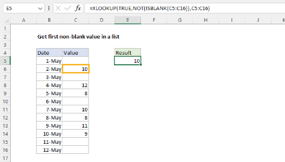
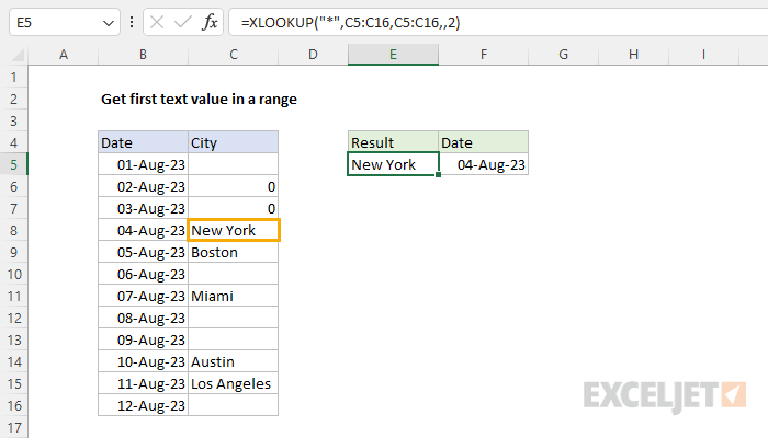
To get the text value in a range you can use the XLOOKUP function with the asterisk (*) wildcard. In the example shown, the formula in E5 is:
=XLOOKUP("*",C5:C16,C5:C16,,2)
This formula finds the text value in the range C5:C16. After ignoring C5, which is empty, and C6 and C7, which contain zeros, the formula returns "New York" - the first text value in the range.
Note: it is also possible to solve this problem with a more modern array formula based on the ISTEXT function. See below for more information.
Generic formula
=XLOOKUP("*",range,range,,2)
Explanation
The general goal is to return the first text value in a range. Specifically, we have dates in column B and some city names in column C. We want a formula to find the first city listed in the range C5:C16. Because some cells in C5:C16 are empty, and some contain zeros, we need to ignore these cells in the process. This problem can be solved using the XLOOKUP function. In older versions of Excel, you can use the VLOOKUP function or an INDEX and MATCH formula. It is also possible to solve this problem with a more modern array formula based on the ISTEXT function. See below for details
Wildcards in Excel formulas
Some Excel functions support wildcards, which can be used to solve this problem. In this case, the wildcard we want is the asterisk () which will match any one or more characters. It's not obvious from the description, but the asterisk () wildcard will only match text characters. It will ignore empty cells, numbers, and errors.
XLOOKUP function
The XLOOKUP function, a modern upgrade of the VLOOKUP function, offers one solution to this problem. When XLOOKUP is used with wildcards, the generic syntax for required inputs looks like this:
=XLOOKUP(lookup_value,lookup_array,return_array,,match_mode)
Where each argument has the following meaning:
- lookup_value - the value to look for
- lookup_array - the range or array to search within
- return_array - the range or array to return values from
- if_not-found - value to return if no match is found (omitted above)
- match_mode - settings for exact, approximate, and wildcard matching
For more details, see How to use the XLOOKUP function.
In the worksheet shown, the formula in E5 is:
=XLOOKUP("*",C5:C16,C5:C16,,2)
Here are the values provided to XLOOKUP:
- lookup_value - "*" (the wildcard)
- lookup_array - C5:C16
- return_array - C5:C16
- if_not-found - omitted
- match_mode - 2 (to enable wildcard matching)
In this configuration, XLOOKUP ignores the empty cell and zero values in the first three cells and returns "New York", which is the first text value in C5:C16. Although the range in this example is organized vertically, XLOOKUP can be used in the same way with a horizontal range. Also, we can easily adapt this formula to return the date (as seen in F5) like this:
=XLOOKUP("*",C5:C16,B5:B16,,2) // get date
This formula will return the corresponding date from the range B5:B16 that aligns with the first text value in C5:C16 - in this case, 04-Aug-23.
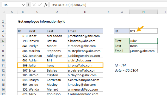
VLOOKUP function
The VLOOKUP function is an older function in Excel widely used for common lookup problems that involve vertical ranges. Like XLOOKUP, VLOOKUP supports wildcards. The generic syntax for VLOOKUP looks like this:
=VLOOKUP(lookup_value,table_array,col_index_num,range_lookup)
Where each argument has the following meaning:
- lookup_value - the value to look for
- table_array - the table to look within
- col_index_num - the number of the column to retrieve
- range_lookup - settings for exact and approximate matching (must be exact for wildcards)
For more details, see How to use the VLOOKUP function.
In the worksheet shown, you can use VLOOKUP to retrieve the first City in the range C5:C16 like this:
=VLOOKUP("*",C5:C16,1,0)
The values provided to VLOOKUP are as follows:
- lookup_value - "*" (the wildcard)
- table_array - C5:C16 (one-column table)
- col_index_num - 1 (first column)
- range_lookup - 0 or FALSE for an exact match (required for wildcards)
In this configuration, VLOOKUP ignores the empty cell and zero values in the first three cells and returns "New York", which is the first text value in C5:C16. Note that VLOOKUP is limited to vertical ranges only. To solve this problem in the same way with a horizontal range you can use the HLOOKUP function. Alternatively, you can use an INDEX and MATCH formula, as explained below.
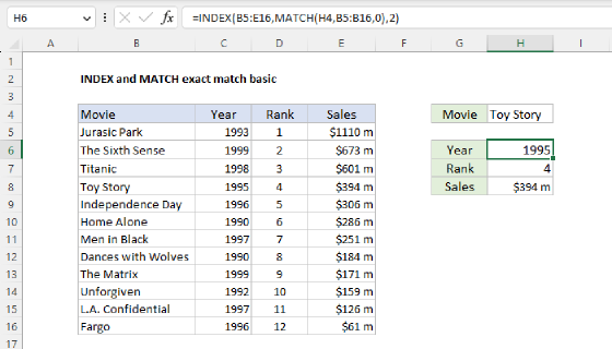
INDEX and MATCH
One problem with VLOOKUP in this problem is that we can't return the date in B5:B16 that corresponds to the first text value in C5:C16. This is one of the limitations of VLOOKUP, which requires the lookup values to be the first column in a table. However, we can use INDEX and MATCH to get both the city and the date like this:
=INDEX(C5:C16,MATCH("*",C5:C16,0)) // get city
=INDEX(B5:B16,MATCH("*",C5:C16,0)) // get date
The approach is the same as with XLOOKUP and VLOOKUP above - we are using MATCH with the (*) wildcard to find the first text value. The location is then provided to INDEX, which returns the final result.
For more details on INDEX with MATCH, see: How to use INDEX and MATCH.
Array formula approach
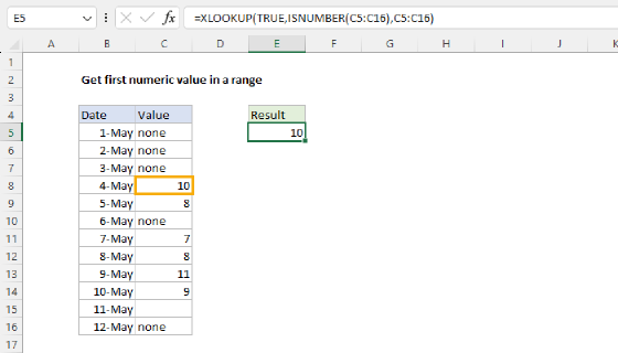
A more modern and flexible way to solve this problem is with an array formula that uses the ISTEXT function. With XLOOKUP, you can use a formula like this:
=XLOOKUP(TRUE,ISTEXT(C5:C16),C5:C16,,2)
In a nutshell, we use the ISTEXT function to test the values in C5:C16 and return an array of TRUE and FALSE values. We then configure XLOOKUP to search this array for the first TRUE value. This is a more flexible approach because it can be easily adapted to test for other types of content, like numbers, errors, and even blank cells. For a more complete explanation, see this example.