Explanation
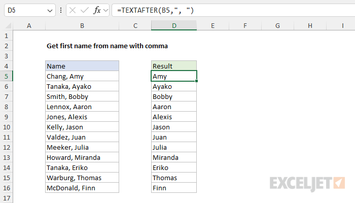
In this example, the goal is to extract the first name from a list of names in "Last, First" format as seen in column B. There are several ways to approach this problem. In the current version of Excel, the easiest solution is to use the TEXTAFTER function. In older versions of Excel, it can be solved with a more complex formula based on the RIGHT, LEN, and FIND functions. Both approaches are explained below.
Modern solution
In the current version of Excel, the TEXTAFTER function is the best way to solve this problem. TEXTAFTER extracts text that occurs after a given delimiter. In its simplest form, TEXTAFTER only requires two arguments, text and delimiter:
=TEXTAFTER(text,delimiter)
In the worksheet shown, the formula we are using to return the last name looks like this:
=TEXTAFTER(B5,", ")
- text - B5, the name in column B
- delimiter - ", " (a comma followed by a single space)
In this configuration, the TEXTAFTER function simply returns all text that appears after the comma and space. If the space character is not consistent (i.e. sometimes the comma is followed by a space, and sometimes not) you can provide more than one delimiter to TEXTAFTER to handle both situations like this:
=TEXTAFTER(B8,{", ",","})
The curly braces indicate an array constant, which is a way to pass more than one value into a function. TEXTAFTER has many other options that you can read more about here.
Legacy solution
In older versions of Excel that do not provide the TEXTAFTER function, you can solve this problem with a more complex formula based on the RIGHT, LEN, and FIND functions:
=RIGHT(B5,LEN(B5)-FIND(",",B5)-1)
As the formula is copied down, it returns the first name from each name in column B. This formula achieves the same result but in a more manual way. At the core, the RIGHT function is used to extract the first name from the full name in column B, starting from the right. The RIGHT function takes two arguments, the text itself and num_chars, which specifies how many characters to extract:
=RIGHT(text,num_chars)
For example, if we use "apple" for text and 3 for num_chars, we get "ple":
=RIGHT("apple",3) returns "ple"
The complexity in the formula comes from working out how many characters to extract, which is done with the snippet below:
LEN(B5)-FIND(",",B5)-1
The challenge problem is to calculate the length of the first name. To work this out, we locate the position of the comma (",") in the text, then we subtract this location from the total length of the text:
LEN(B5)-FIND(",",B5)-1
The LEN function calculates the total characters in the text:
LEN(B5) // returns 10
Because there are ten characters in "Chang, Amy", LEN returns 10. Next, the FIND function is used to locate the comma (",") in the text:
=FIND(",",B5) // returns 6
Because the comma (",") occurs as the sixth character in the text, FIND returns 6. When we subtract 6 from 10, we get 4:
=LEN(B5)-FIND(",",B5)
=10-6
=4
This is close to what we need, but "Amy" contains 3 characters, not 4 characters. If we ask RIGHT for the last 4 characters in "Chang, Amy", we'll also get the space that follows the comma. So, we need to subtract 1 to take the comma into account:
=LEN(B5)-FIND(",",B5)-1
=10-6-1
=3
The code above returns this result directly to the RIGHT function as the num_chars argument:
RIGHT("Chang, Amy",3) // returns "Amy"
And RIGHT returns "Amy" as the final result.
Note: If there is no space after the comma, there is no need to subtract 1.
Get the last name
To extract the last name from the names in column B, you can use a similar formula based on the LEFT function:
=LEFT(B5,FIND(",",B5)-1)
See the example here for a full explanation.


