Summary
To get the day name (i.e. Monday, Tuesday,Wednesday, etc.) from a date, you can use the TEXT function. In the example shown, the formula in cell C5 is:
=TEXT(B5,"dddd")
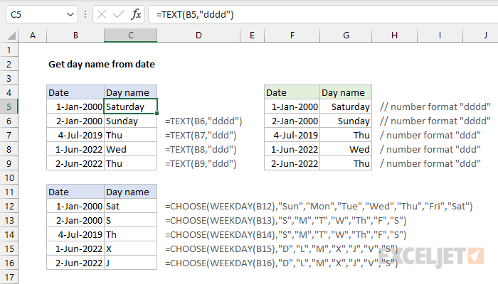
With January 1, 2000, in cell B5, the TEXT function returns the text string "Saturday".
Generic formula
TEXT(A1,"dddd")
Explanation
In this example, the goal is to get the day name (i.e. Monday, Tuesday, Wednesday, etc.) from a given date. There are several ways to go about this in Excel, depending on your needs. This article explains three approaches:
- Display date with a custom number format
- Convert date to day name with TEXT function
- Convert date to day name with CHOOSE function
For all examples, keep in mind that Excel dates are large serial numbers, displayed as dates with number formatting.
Day name with custom number format
To display a date using only the day name, you don't need a formula; you can just use a custom number format. Select the date, and use the shortcut Control + 1 to open Format cells. Then select Number > Custom, and enter one of these custom formats:
"ddd"  // i.e."Wed"
"dddd" // i.e."Wednesday"
Excel will display only the day name, but it will leave the date intact. If you want to display both the date and the day name in different columns, one option is to use a formula to pick up a date from another cell and change the number format to show only the day name. For example, in the worksheet shown, cell F5 contains the date January 1, 2000. The formula in G5, copied down, is:
=F5 // get date from F5
Cells G5 and G6 have the number format "dddd" applied, and cells in G7:G9 have the number format "ddd" applied.
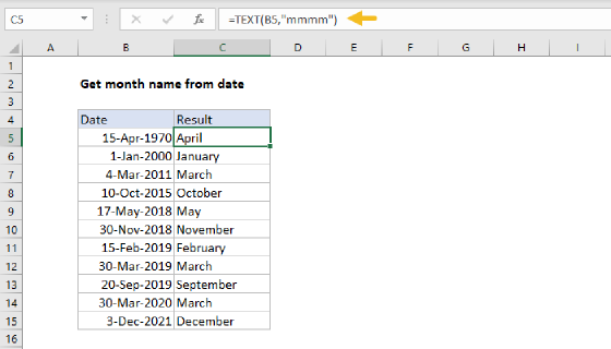
Day name with the TEXT function
To convert a date to a text value like "Saturday", you can use the TEXT function. The TEXT function is a general function that can be used to convert numbers of all kinds into text values with formatting, including date formats. For example, with the date January 1, 2000, in cell A1, you can use TEXT like this:
=TEXT(A1,"d-mmm-yyyy") // returns "1-Jan-2000"
=TEXT(A1,"mmmm d, yyyy") // returns "January 1, 2000"
=TEXT(A1,"mmmm") // returns "January"
In the worksheet shown, the goal is to display the day name only, so we use a custom number format like "ddd" or "dddd":
=TEXT(B5,"dddd") // returns "Saturday"
=TEXT(B5,"ddd") // returns "Sat"
Note: The TEXT function converts a date to a text value using the supplied number format. The date is lost in the conversion and only the text for the day name remains.
Day name with CHOOSE function
For maximum flexibility, you can create your own day names with the CHOOSE function. CHOOSE is a general-purpose function for returning a value based on a numeric index. For example, you can use CHOOSE to return one of three colors with a number like this:
=CHOOSE(1,"red","blue","green") // returns "red"
=CHOOSE(2,"red","blue","green") // returns "blue"
=CHOOSE(3,"red","blue","green") // returns "green"
In this example, the goal is to return a day name from a date, so we need to configure CHOOSE to select one of the seven-day names. For example, the formula below would return "Wed" based on a numeric index of 4:
=CHOOSE(4,"Sun","Mon","Tue","Wed","Thu","Fri","Sat") // "Wed"
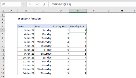
The challenge, in this case, is to get the right index for a date and for that we need the WEEKDAY function. For any given date, WEEKDAY returns a number between 1-7, which corresponds to the day of the week. By default, WEEKDAY returns 1 for Sunday, 2 for Monday, 3 for Tuesday, etc. In the worksheet shown, the formula in C12 is:
=CHOOSE(WEEKDAY(B12),"Sun","Mon","Tue","Wed","Thu","Fri","Sat")
WEEKDAY returns a number between 1-7, and CHOOSE will use this number to select the corresponding value in the list. Since the date in B12 is January 1, 2000, WEEKDAY returns 7, and CHOOSE returns "Sat".
CHOOSE is more work to set up, but it is also more flexible since it allows you to convert a date to a day name using any values you want. For example, you can use custom abbreviations or even abbreviations in a different language. In cell C15, CHOOSE is set up to use one-letter abbreviations that correspond to Spanish day names:
=CHOOSE(WEEKDAY(B15),"D","L","M","X","J","V","S")
Empty cells
If you use the formulas above on an empty cell, you'll get "Saturday" as the result. This happens because an empty cell is evaluated as zero, and zero in the Excel date system is the date "0-Jan-1900", which is a Saturday. To work around this issue, you can use the IF function to return an empty string ("") for empty cells. For example, if cell A1 may or may not contain a date, you can use IF like this:
=IF(A1<>"",TEXT(A1,"ddd"),"") // check for empty cells
The literal translation of this formula is: If A1 is not empty, return the TEXT formula, otherwise return an empty string ("").