Summary
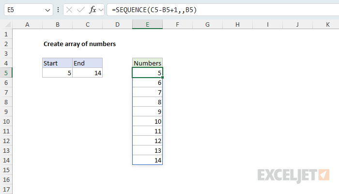
To create an array of numbers like {1;2;3;4;5}, you can use the SEQUENCE function. In the example shown, the formula in E5 is:
=SEQUENCE(C5-B5+1,,B5)
The result is an array of the 10 numbers from 5 to 14, which spills into E5:E14. SEQUENCE is available in Excel 2021+ and Excel 365. For a formula that works in any version of Excel, you can use the ROW and INDIRECT functions:
=ROW(INDIRECT(B5&":"&C5))
See below for details on both formulas.
Generic formula
=SEQUENCE(end-start+1,,start)
Explanation
In this example, the goal is to create an array of numbers from a start value in B5 to an end value in C5. An array like this is most often used inside a larger formula that needs a numeric array for processing of some kind. The worksheet shows the result as a spill so you can see the numbers.
SEQUENCE function
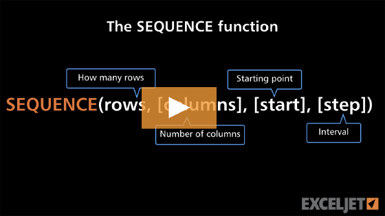
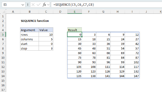
The SEQUENCE function generates a list of numbers. It takes four arguments, rows, columns, start, and step, and only rows is required. SEQUENCE doesn't take an end value. Instead, it needs the count of numbers to return, so the formula calculates the count from the start and end values:
C5-B5+1 // 14-5+1 = 10
The 1 is needed because both the start and end values are included. columns is left empty, so the result is a single column. start is B5, and step is omitted, so it defaults to 1:
=SEQUENCE(10,,5) // returns {5;6;7;8;9;10;11;12;13;14}
Because SEQUENCE takes the start value directly, negative numbers and zero work too. With -5 in B5 and 5 in C5, the formula returns {-5;-4;-3;-2;-1;0;1;2;3;4;5}.
Other arrays of numbers
To create other arrays, change the arguments:
=SEQUENCE(10) // 1 to 10
=SEQUENCE(C5-B5+1,,C5,-1) // end to start, descending
=SEQUENCE(1,C5-B5+1,B5) // start to end, in one row
=SEQUENCE((C5-B5)/5+1,,B5,5) // start to end, in steps of 5
To count down, start at the end value in C5 and use a step of -1. If the end value is less than the start value, the count is negative and SEQUENCE returns #VALUE!. For more options, including grids, dates, and times, see the SEQUENCE function page.
Arrays inside other formulas
An array of numbers usually isn't the final result. More often, it feeds another function that needs to do something once for each number:
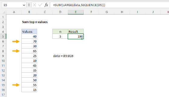
=SUM(LARGE(data,SEQUENCE(3))) // sum the top 3 values
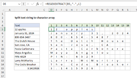
=MID(B5,SEQUENCE(LEN(B5)),1) // split text into characters
In the first formula, SEQUENCE returns {1;2;3}, so LARGE returns the 1st, 2nd, and 3rd largest values, and SUM adds them up. In the second formula, LEN returns the number of characters in B5, and MID extracts one character at each position. For details, see Sum top n values and Split text string to character array.
ROW and INDIRECT
In older versions of Excel without SEQUENCE, you can create an array of numbers with the ROW and INDIRECT functions. This formula works in any version of Excel:
=ROW(INDIRECT(B5&":"&C5))
The core of this formula is a string that represents rows. For example, to create an array with 10 numbers, you can hard-code a string into INDIRECT like this:
=ROW(INDIRECT("1:10"))
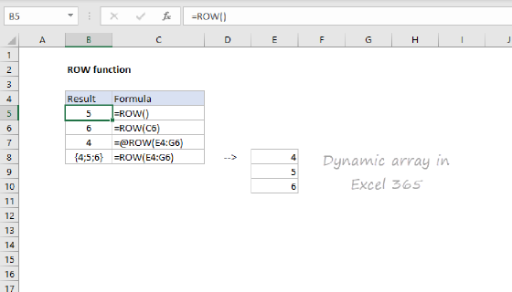
The INDIRECT function interprets this text to mean the range 1:10 (10 rows) and the ROW function returns the row number for each row in that range inside an array.
The example shown picks up the start and end numbers from B5 and C5 respectively, so the solution looks like this:
=ROW(INDIRECT(B5&":"&C5))
=ROW(INDIRECT(5&":"&14))
=ROW(INDIRECT("5:14"))
=ROW(5:14)
={5;6;7;8;9;10;11;12;13;14}
The reason INDIRECT is used in the formula is to guard against worksheet changes. Without INDIRECT, inserting or deleting rows can change the range reference, for example:
=ROW(1:5)
will change to:
=ROW(1:4)
If row 1 is deleted. Because INDIRECT works with a reference constructed with text, it isn't affected by changes on the worksheet.
In Excel 2019 and older, this formula displays only the first number when entered in a single cell. Use F9 in the formula bar to see the actual array result. Normally, you will use this formula inside a larger array formula, entered with Control + Shift + Enter.
This approach has some limitations. Row numbers start at 1, so ROW won't return zero or negative numbers (INDIRECT returns #REF!), and you need math to shift or reverse the array:
=ROW(INDIRECT(1&":"&5))-6 // returns {-5;-4;-3;-2;-1}
=ABS(ROW(INDIRECT("1:"&n))-(n+1)) // returns n to 1
If the end value is less than the start value, the formula quietly returns the numbers in ascending order anyway, because "14:5" refers to the same rows as "5:14". INDIRECT is also a volatile function, so any formula that uses it recalculates whenever anything in the workbook changes.
Relative row numbers in a range
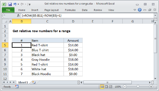
If you need an array of the relative row numbers in a range ({1;2;3;...}, one number per row), give SEQUENCE the number of rows in the range:
=SEQUENCE(ROWS(range))
In any version of Excel, you can use a formula like this:
=ROW(range)-ROW(range.firstcell)+1
See this page for a full explanation.