Summary
To count visible rows with criteria, you can use a rather complex formula based on three main functions: SUMPRODUCT, SUBTOTAL, and OFFSET. In the example shown, the formula in H7 is:
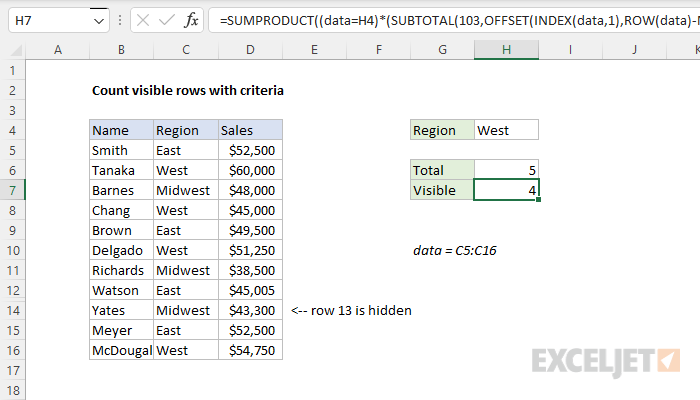
=SUMPRODUCT((data=H4)*(SUBTOTAL(103,OFFSET(INDEX(data,1),ROW(data)-MIN(ROW(data)),0))))
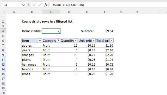
Where data is the named range C5:C16. The result is 4 since there are four visible rows where the Region is "West".
Generic formula
=SUMPRODUCT((criteria)*(SUBTOTAL(103,OFFSET(range,rows,0,1))))
Explanation
In this example, the goal is to count visible rows where Region="West". Row 13 meets this criteria, but has been hidden. The SUBTOTAL function can easily generate sums and counts for visible rows. However, SUBTOTAL is not able to apply criteria like the COUNTIFS function without help. Conversely, COUNTIFS can easily apply criteria but is not able to distinguish between rows that are visible and rows that are hidden. One solution is to use Boolean logic to apply criteria, then use the SUBTOTAL function together with the OFFSET function to check visibility, and then tally up results with the SUMPRODUCT function. The details of this approach are described below.
Overview
At the core, this formula works by setting up two arrays inside SUMPRODUCT. The first array applies criteria, and the second array handles visibility:
=SUMPRODUCT(criteria*visibility)
The formula in H7 takes this approach:
=SUMPRODUCT((data=H4)*(SUBTOTAL(103,OFFSET(INDEX(data,1),ROW(data)-MIN(ROW(data)),0))))
Criteria
The criteria are applied with this part of the formula:
=(data=H4)
Because there are 12 values in data (C5:C16) this expression generates an array with 12 TRUE and FALSE results like this:
{FALSE;TRUE;FALSE;TRUE;FALSE;TRUE;FALSE;FALSE;TRUE;FALSE;FALSE;TRUE}
The TRUE values in this array indicate cells in data that contain "West". When this array is multiplied by the array returned by the SUBTOTAL function (described in detail below) the math operation coerces the TRUE and FALSE values to 1s and 0s, which creates this final array of results:
{0;1;0;1;0;1;0;0;1;0;0;1}
This array is used to apply the criteria Region="West" in one of the last steps below.
Visibility
To check visibility, we use an expression like this:
(SUBTOTAL(103,OFFSET(INDEX(data,1),ROW(data)-MIN(ROW(data)),0)))
At a high level, we are using the SUBTOTAL function with function_num set to 103, which causes SUBTOTAL to count visible cells, ignoring cells that are hidden with a filter, or hidden manually. The reason the expression is complex is that we need an array of results, not a single result. This means we need to feed cells into SUBTOTAL one at a time using the OFFSET function. To do this, we have configured OFFSET to create the references needed for ref1 inside SUBTOTAL like this:
OFFSET(INDEX(data,1),ROW(data)-MIN(ROW(data)),0)
Working from the inside out, reference is provided to OFFSET with the INDEX function like this:
INDEX(data,1) // first cell in data
We are simply asking INDEX for the first cell in the named range data, and INDEX (under the hood) returns C5 as a result:
OFFSET(C5,ROW(data)-MIN(ROW(data)),0)
The rows argument inside of OFFSET is created like this:
=ROW(data)-MIN(ROW(data))
={5;6;7;8;9;10;11;12;13;14;15;16}-5
={0;1;2;3;4;5;6;7;8;9;10;11}
Essentially, we are using this construction to create a zero-based index of offsets to give to the OFFSET function:
OFFSET(C5,{0;1;2;3;4;5;6;7;8;9;10;11},0)
Using these 12 row offsets, the OFFSET function returns an array of 12 cell references like this:
{C5;C6;C7;C8;C9;C10;C11;C12;C13;C14;C15;C16}
This array of references is returned to the SUBTOTAL function as the ref1 argument:
(SUBTOTAL(103,{C5;C6;C7;C8;C9;C10;C11;C12;C13;C14;C15;C16}))
With function_num set to 103, SUBTOTAL returns the count of visible cells in each reference. Because each reference is provided separately, we get back an array with 12 counts like this:
{1;1;1;1;1;1;1;1;0;1;1;1}
Since we are feeding the references to SUBTOTAL one at a time, the only possible values are 1 and 0, which is exactly what we need when we multiply this array by the array we created for the criteria below. To recap, the complexity above is needed to get to 12 results instead of the single result SUBTOTAL would give us if we provided a simple range.
Adding up results
Finally, we are ready to add up the results. For this, we use the SUMPRODUCT function. Both arrays explained above are delivered to SUMPRODUCT like this:
=SUMPRODUCT({0;1;0;1;0;1;0;0;1;0;0;1}*{1;1;1;1;1;1;1;1;0;1;1;1})
After the two arrays are multiplied, we have:
=SUMPRODUCT({0;1;0;1;0;1;0;0;0;0;0;1}) // returns 4
In the final step, SUMPRODUCT sums the array and returns 4 as a final result.
Multiple criteria
You can extend the formula to handle multiple criteria like this:
=SUMPRODUCT((criteria1)*(criteria2)*(SUBTOTAL(103,OFFSET(ref,rows,0,1))))
Summing results
To return a sum of visible values (instead of a count), you can adapt the formula to include a range of cells to sum like this:
=SUMPRODUCT(criteria*visibility*sumrange)
The sum range is the range that contains values you want to sum. The criteria and visibility arrays work the same as explained above, excluding cells that are not visible. If you need partial matching, you can construct an expression using ISNUMBER + SEARCH, as explained here, to create the criteria array.