Summary
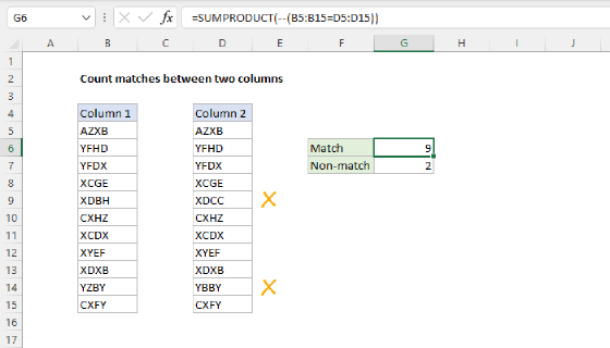
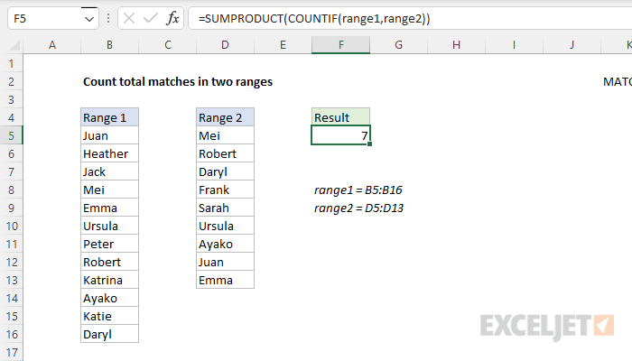
To count total matches in two ranges, you can use a formula that combines the COUNTIF function with the SUMPRODUCT function. In the example shown, the formula in cell F5 is:
=SUMPRODUCT(COUNTIF(range1,range2))
where range1 (B5:B16) and range2 (D5:D13) are named ranges.
Note: this formula does not care about the location or order of the items in each range.
Generic formula
=SUMPRODUCT(COUNTIF(range1,range2))
Explanation
In this example, the goal is to count the number of exact matches in two ranges, ignoring the sort order or location of the values in each range. This problem can be solved with the COUNTIF function or with the MATCH function. Each approach is explained below.
Note: Both formulas below use the SUMPRODUCT function to "tally up" the final count, because SUMPRODUCT handles arrays natively in Legacy Excel. In the current version of Excel, which supports dynamic arrays, you can use the SUM function instead.
COUNTIF function
The COUNTIF function counts values in a range that meet supplied criteria. Normally, you would give COUNTIF a range like A1:A10 and criteria like "red":
=COUNTIF(A1:A10,"red") // count "red" cells
COUNTIF would then return a count of cells in A1:A10 that are equal to "red". In this case, however, we are giving COUNTIF a range of values for criteria, which causes COUNTIF to return a count for each value. The formula in cell F5 is:
=SUMPRODUCT(COUNTIF(range1,range2))
Working from the inside out, we provide range1 (B5:B16) for range and range2 (D5;D13) for criteria:
COUNTIF(range1,range2)
Because we are giving COUNTIF a range that contains 9 values for criteria, COUNTIF will return 9 counts in an array like this:
{1;1;1;0;0;1;1;1;1}
Each item in this array represents a count. A positive number represents the count of a value in range2 that was found in range1. A zero indicates a value that was not found. COUNTIF returns this array of counts directly to the SUMPRODUCT function:
=SUMPRODUCT({1;1;1;0;0;1;1;1;1}) // returns 7
With just one array to process, SUMPRODUCT sums the array and returns 7 as a final result.
MATCH function
Another way to solve this problem is with the MATCH function like this:
=SUMPRODUCT(--ISNUMBER(MATCH(range1,range2,0)))
Working from the inside out, the MATCH function is configured with range1 as lookup_value, range2 as lookup_array, and match_type as 0 for an exact match.:
MATCH(range1,range2,0)
Because we are asking MATCH to find 12 values, we get back an array with 12 results like this:
{8;#N/A;#N/A;1;9;6;#N/A;2;#N/A;7;#N/A;3}
In this array, a number represents the position of a matched value, and the #N/A error indicates a value that was not found. To convert this array to TRUE and FALSE values, we use the ISNUMBER function:
--ISNUMBER({8;#N/A;#N/A;1;9;6;#N/A;2;#N/A;7;#N/A;3})
ISNUMBER returns TRUE for any number and FALSE for anything else, so the resulting array looks like this:
{TRUE;FALSE;FALSE;TRUE;TRUE;TRUE;FALSE;TRUE;FALSE;TRUE;FALSE;TRUE}
By default, the SUMPRODUCT function will ignore the logical values TRUE and FALSE, so we use a double negative (--) to convert the TRUE and FALSE values to 1s and 0s. The resulting array is returned to the SUMPRODUCT function:
=SUMPRODUCT({1;0;0;1;1;1;0;1;0;1;0;1}) // returns 7
With only one array to process, SUMPRODUCT sums the array and returns a final result of 7.
MATCH with COUNT
As I mentioned above, in the current version of Excel, which supports dynamic array formulas, you can use the SUM function instead of the SUMPRODUCT function like this:
=SUM(--ISNUMBER(MATCH(range1,range2,0)))
The reason SUMPRODUCT is traditionally used is that it avoids the requirement of entering the formula as an array formula with control + shift + enter in older versions of Excel. However, an interesting result of dynamic arrays in Excel is that they make new solutions possible, because the native array behavior affects older functions as well. For example, in the current version of Excel, we can use the COUNT function directly like this:
=COUNT(MATCH(range1,range2,0))
COUNT is programmed to count only numeric values — it returns the count of numbers in the array returned by MATCH and simply ignores the #N/A errors. The formula evaluates like this:
=COUNT(MATCH(range1,range2,0))
=COUNT({8;#N/A;#N/A;1;9;6;#N/A;2;#N/A;7;#N/A;3})
=7
To be clear, this formula will also work in older versions of Excel. However, it must be entered as an array formula with control + shift + enter. In the current version of Excel, it just works.
Match across rows
The formulas above do not care about the location of values in the two ranges. If you want to compare two ranges and count matches at the row level (i.e. only count matches when the same item appears in the same position), you'll need a different formula.