Summary
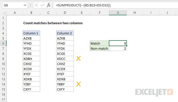
To compare two columns and count matches in corresponding rows, you can use the SUMPRODUCT function. In the example shown, the formula in G6 is:
=SUMPRODUCT(--(B5:B15=D5:D15))
The result is 9 because there are nine values in the range B5:B15 that match values in D5:D15 in corresponding rows.
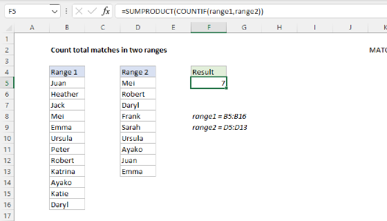
Note: this formula counts matches in corresponding rows. To count all matches in two ranges, regardless of row, see this example.
Generic formula
=SUMPRODUCT(--(range1=range2))
Explanation
In this example, the goal is to compare two columns and return the count of matches in corresponding rows. A good way to solve this problem is to use the SUMPRODUCT function or the SUM function, as explained below.
SUMPRODUCT function
The SUMPRODUCT function is a versatile function that handles array operations natively without any special array syntax. Its behavior is simple: it multiplies, then sums the product of arrays. Working from the inside out, we compare the range B5:B15 to D5:D15 like this:
B5:B15=D5:D15
Because there are 11 values in the first range, the result is an array with 11 TRUE and FALSE values like this:
{TRUE;TRUE;TRUE;TRUE;FALSE;TRUE;TRUE;TRUE;TRUE;FALSE;TRUE}
In this array, the TRUE values correspond to cells in B5:B15 that match corresponding cells in D5:D15. In this state, SUMPRODUCT will actually return zero because TRUE and FALSE values are not counted as numbers in Excel by default. To get SUMPRODUCT to treat TRUE as 1 and FALSE as zero, we need to "coerce" them into numbers. The double negative (--) is a simple way to do that:
--(B5:B15=D5:D15)
This results in an array containing only 1s and 0s, which is returned directly to the SUMPRODUCT function:
=SUMPRODUCT({1;1;1;1;0;1;1;1;1;0;1}) // returns 9
With no other arrays to multiply, SUMPRODUCT simply sums the values and returns 9.
Count non-matching rows
To count non-matching values, you can reverse the logic and use the not equal to operator (<>). The formula in G7 is:
=SUMPRODUCT(--(B5:B15<>D5:D15))
This formula returns 2, since there are two non-matching cells.
SUM function
Traditionally, the SUMPRODUCT function has been used instead of the SUM function in Legacy Excel, because SUMPRODUCT can handle array operations without Control + Shift + Enter. In Excel 365 and Excel 2021, the formula engine handles array formulas natively, so you can use the SUM function instead without special treatment:
=SUM(--(B5:B15=D5:D15)) // count matches
=SUM(--(B5:B15<>D5:D15)) // count non-matches
For more details, see this article.