Summary
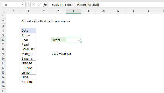
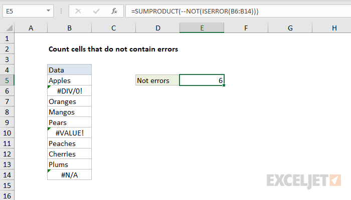
To count the number of cells that do not contain errors, you can use the ISERROR and NOT functions, wrapped in the SUMPRODUCT function. In the example shown, the formula in E5 is:
=SUMPRODUCT(--NOT(ISERROR(B5:B14)))
The result is 7, since there are seven cells in B5:B14 that do not contain error values.
Generic formula
=SUMPRODUCT(--NOT(ISERROR(range)))
Explanation
In this example, the goal is to count the number of cells in a range that do not contain errors. The best way to solve this problem is to use the SUMPRODUCT function together with the ISERROR function. You can also use the COUNTIF function or COUNTIFS function to exclude specific errors. Both approaches are explained below.
COUNTIF function
One way to count cells that do not contain errors is to use the COUNTIF function like this:
=COUNTIF(B5:B14,"<>#N/A") // returns 9
For criteria, we use the not equal to operator (<>) with #N/A. Notice both values are enclosed in double quotes. COUNTIF returns 9 since there are nine cells in B5:B15 that do not contain the #N/A error. If we switch to the COUNTIFS function, we can exclude more than one kind of error like this:
=COUNTIFS(B5:B14,"<>#N/A",B5:B14,"<>#VALUE!") // returns 8
COUNTIFS returns 9 since there are eight cells in B5:B15 that do not contain the #N/A error or the #VALUE! error. However, this approach is tedious if the goal is to exclude all types of errors from the count. In that case, the SUMPRODUCT option below is more straightforward.
SUMPRODUCT function
The SUMPRODUCT function works directly with arrays and ranges. One thing you can do quite easily with SUMPRODUCT is perform a logical test on a range, then count the results. In this case, we want to count cells that do not contain errors and the simplest way to do that is with the ISERROR function and the NOT function. In the worksheet shown above, the formula in cell E5 is:
=SUMPRODUCT(--NOT(ISERROR(B5:B14)))
Working from the inside out, we first use the ISERROR function on the range B5:B14.
ISERROR(B5:B14) // check all 10 cells
Since there are ten cells in the range B5:B14, ISERROR returns an array with ten results like this:
{FALSE;TRUE;FALSE;FALSE;FALSE;TRUE;FALSE;FALSE;FALSE;TRUE}
Here, each TRUE value indicates a cell value that is an error. Since the goal is to count cells that do not contain errors, we reverse these results with the NOT function:
NOT({FALSE;TRUE;FALSE;FALSE;FALSE;TRUE;FALSE;FALSE;FALSE;TRUE})
which returns a new array like this:
{TRUE;FALSE;TRUE;TRUE;TRUE;FALSE;TRUE;TRUE;TRUE;FALSE}
Notice that each TRUE value now corresponds to a cell that does not contain an error. This array is now in the correct form. However, SUMPRODUCT only works with numeric data so the next step is to convert the TRUE and FALSE values to their numeric equivalents, 1 and 0. We do this with a double negative (--):
--{TRUE;FALSE;TRUE;TRUE;TRUE;FALSE;TRUE;TRUE;TRUE;FALSE}
The resulting array looks like this:
{1;0;1;1;1;0;1;1;1;0}
Finally, SUMPRODUCT sums the items in this array and returns the total, which in the example is the number 3:
=SUMPRODUCT({1;0;1;1;1;0;1;1;1;0}) // returns 7
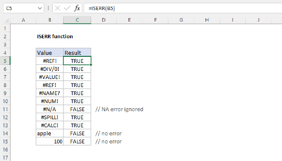
ISERR function
Like the ISERROR function, the ISERR function returns TRUE when a value is an error. The difference is that ISERR ignores #N/A errors. If you want to count cells that do not contain errors, and ignore #N/A errors, you can substitute ISERR for ISERROR:
=SUMPRODUCT(--NOT(ISERR(B5:B14))) // returns 8
SUMPRODUCT returns 8 since there are eight cells that do not contain errors, ignoring the #N/A error in cell B14.