Summary
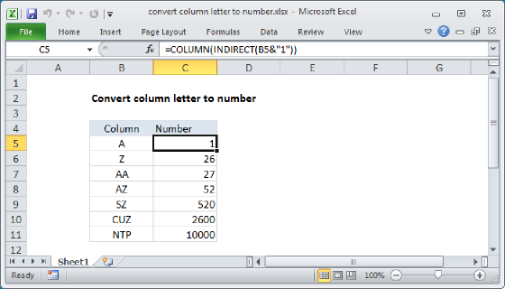
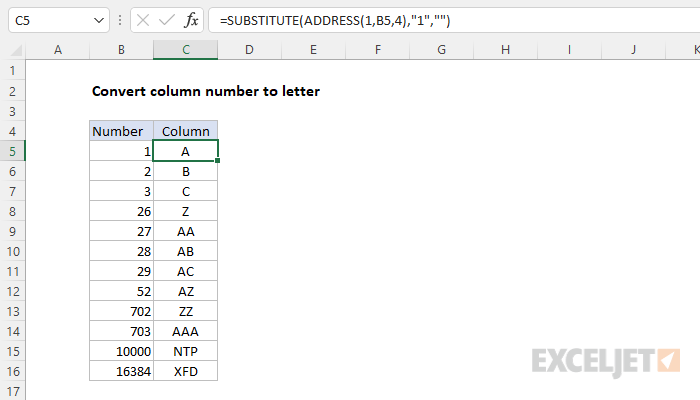
To convert a column number to an Excel column letter (e.g. A, B, C, etc.) you can use a formula based on the ADDRESS and SUBSTITUTE functions. In the example shown, the formula in C5, copied down, is:
=SUBSTITUTE(ADDRESS(1,B5,4),"1","")
The result is the column reference as one or more letters, returned as a text string.
Generic formula
=SUBSTITUTE(ADDRESS(1,number,4),"1","")
Explanation
In this example, the goal is to convert an ordinary number into a column reference expressed in letters. For example, the number 1 should return "A", the number 2 should return "B", the number 26 should return "Z", etc. The challenge is that Excel can handle over 16,000 columns, so the number of letter combinations is large. One way to solve this problem is to construct a valid address with the number and extract just the column from the address. This is the approach explained below. For reference, the formula in C5 is:
=SUBSTITUTE(ADDRESS(1,B5,4),"1","")
ADDRESS function
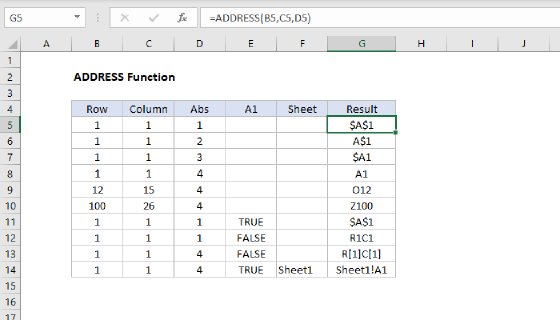
Working from the inside out, the first step is to construct an address that contains the correct column reference. We can do this with the ADDRESS function, which will return the address for a cell based on a given row and column number. For example:
=ADDRESS(1,1) // returns "$A$1"
=ADDRESS(1,2) // returns "$B$1"
=ADDRESS(1,26) // returns "$Z$1"
By providing 4 for the optional abs_num argument, we can get a relative reference:
=ADDRESS(1,1,4) // returns "A1"
=ADDRESS(1,2,4) // returns "B1"
=ADDRESS(1,26,4) // returns "Z1"
Note the result from ADDRESS is always a text string. We don't particularly care about the row number, we only care about the column number, so we use 1 for row_num in all cases. In the worksheet shown, we get the column number from column B and use 1 for the row number like this:
ADDRESS(1,B5,4)
As the formula is copied down, ADDRESS creates a valid address using each number in column B. The maximum number of columns in an Excel worksheet is 16,384, so the final column in a worksheet is "XFD".
SUBSTITUTE function
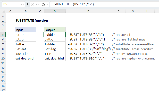
Now that we have an address with the column reference we want, we simply need to remove the row number. One way to do this is with the SUBSTITUTE function. For example, assuming we have an address like "A1", we can use SUBSTITUTE like this:
=SUBSTITUTE("A1","1","") // returns "A"
We are telling SUBSTITUTE to look for "1" and replace it with an empty string (""). We can confidently do this in all cases because we've hardcoded the row number as 1 inside the ADDRESS function. The final formula in C5 is:
=SUBSTITUTE(ADDRESS(1,B5,4),"1","")
In brief, ADDRESS creates the cell reference and returns the result to SUBSTITUTE, which removes the "1".
TEXTBEFORE function
A cleaner way to extract the column reference from the address is to use the TEXTBEFORE function like this:
=TEXTBEFORE(ADDRESS(1,B5,4),"1")
Here, we treat "1" as a delimiter and ask TEXTBEFORE for all text before the delimiter. The result from this formula is the same as above, but the configuration is a bit simpler.