Summary
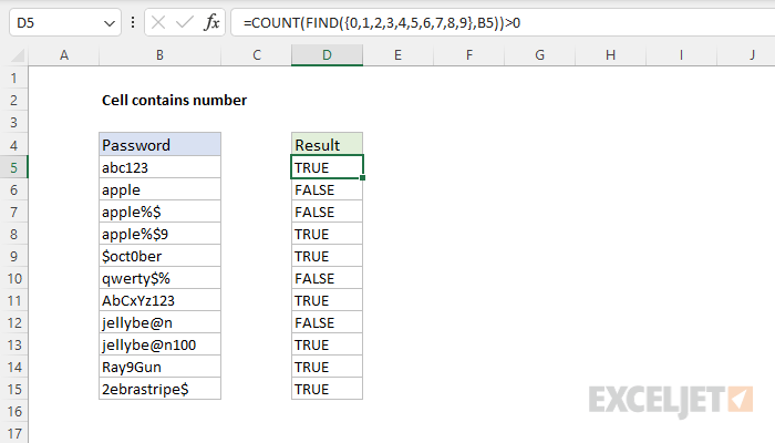
To test if a cell or text string contains a number, you can use the FIND function together with the COUNT function. The numbers to look for are supplied as an array constant. In the example the formula in D5 is:
=COUNT(FIND({0,1,2,3,4,5,6,7,8,9},B5))>0
As the formula is copied down, it returns TRUE if a value contains a number and FALSE if not. See below for an alternate formula based on the SEQUENCE function.
Generic formula
=COUNT(FIND({0,1,2,3,4,5,6,7,8,9},A1))>0
Explanation
In this example, the goal is to test the passwords in column B to see if they contain a number. This is a surprisingly tricky problem because Excel doesn't have a function that will let you test for a number inside a text string directly. Note this is different from checking if a cell value is a number. You can easily perform that test with the ISNUMBER function. In this case, however, we to test if a cell value contains a number, which may occur anywhere. One solution is to use the FIND function with an array constant. In Excel 365, which supports dynamic array formulas, you can use a different formula based on the SEQUENCE function. Both approaches are explained below.
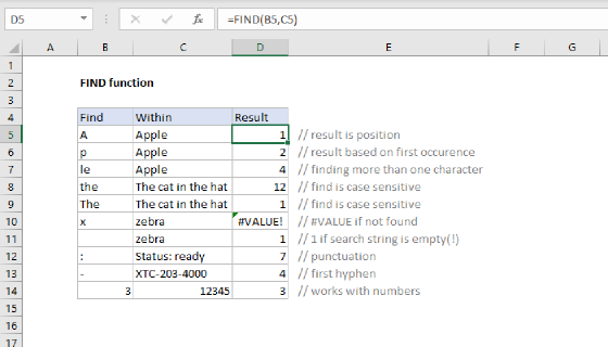
FIND function
The FIND function is designed to look inside a text string for a specific substring. If FIND finds the substring, it returns a position of the substring in the text as a number. If the substring is not found, FIND returns a #VALUE error. For example:
=FIND("p","apple") // returns 2
=FIND("z","apple") // returns #VALUE!
We can use this same idea to check for numbers as well:
=FIND(3,"app637") // returns 5
=FIND(9,"app637") // returns #VALUE!
The challenge in this case is that we need to check the values in column B for ten different numbers, 0-9. One way to do that is to supply these numbers as the array constant {0,1,2,3,4,5,6,7,8,9}. This is the approach taken in the formula in cell D5:
=COUNT(FIND({0,1,2,3,4,5,6,7,8,9},B5))>0
Inside the COUNT function, the FIND function is configured to look for all ten numbers in cell B5:
FIND({0,1,2,3,4,5,6,7,8,9},B5)
Because we are giving FIND ten values to look for, it returns an array with 10 results. In other words, FIND checks the text in B5 for each number and returns all results at once:
{#VALUE!,4,5,6,#VALUE!,#VALUE!,#VALUE!,#VALUE!,#VALUE!,#VALUE!}
Unless you look at arrays often, this may look pretty cryptic. Here is the translation: The number 1 was found at position 4, the number 2 was found at position 5, and the number 3 was found at position 6. All other numbers were not found and returned #VALUE errors.
We are very close now to a final formula. We simply need to tally up results. To do this, we nest the FIND formula above inside the COUNT function like this:
=COUNT(FIND({0,1,2,3,4,5,6,7,8,9},B5))
FIND returns the array of results directly to COUNT, which counts the numbers in the array. COUNT only counts numeric values, and ignores errors. This means COUNT will return a number greater than zero if there are any numbers in the value being tested. In the case of cell B5, COUNT returns 3.
The last step is to check the result from COUNT and force a TRUE or FALSE result. We do this by adding ">0" to the end of formula:
=COUNT(FIND({0,1,2,3,4,5,6,7,8,9},B5))>0
Now the formula will return TRUE or FALSE. To display a custom result, you can use the IF function:
=IF(COUNT(FIND({0,1,2,3,4,5,6,7,8,9},B5))>0, "Yes", "No")
The original formula is now nested inside IF as the logical_test argument. This formula will return "Yes" if B5 contains a number and "No" if not.
SEQUENCE function
In Excel 365, which offers dynamic array formulas, we can take a different approach to this problem.
=COUNT(--MID(B5,SEQUENCE(LEN(B5)),1))>0
This isn't necessarily a better approach, just a different way to solve the same problem. At the core, this formula uses the MID function together with the SEQUENCE function to split the text in cell B5 into an array:
MID(B5,SEQUENCE(LEN(B5)),1)
Working from the inside out, the LEN function returns the length of the text in cell B5:
LEN(B5) // returns 6
This number is returned to the SEQUENCE function as the rows argument, and SEQUENCE returns an array of numbers, 1-6:
=SEQUENCE(LEN(B5))
=SEQUENCE(6)
={1;2;3;4;5;6}
This array is returned to the MID function as the start_num argument, and, with num_chars set to 1, the MID function returns an array that contains the characters in cell B5:
=MID(B5,{1;2;3;4;5;6},1)
={"a";"b";"c";"1";"2";"3"}
We can now simplify the original formula to:
=COUNT(--{"a";"b";"c";"1";"2";"3"})>0
We use the double-negative (--) to get Excel to try and coerce the values in the array into numbers. The result looks like this:
=COUNT({#VALUE!;#VALUE!;#VALUE!;1;2;3})>0
The math operation created by the double negative (--) returns an actual number when successful and a #VALUE! error when the operation fails. The COUNT function counts the numbers, ignoring any errors, and returns 3. As above, we check the final count with ">0", and the result for cell B5 is TRUE.
Note: as you might guess, you can easily adapt this formula to count numbers in a text string.
Cell equals number?
Note that the formulas above are too complex if you only want to test if a cell equals a number. In that case, you can simply use the ISNUMBER function like this:
=ISNUMBER(A1)