
Summary
Data validation can help control what a user can enter into a cell. You can use data validation to make sure a value is a number, a date, or to present a dropdown menu with predefined choices to a user. This guide provides an overview of the data validation feature, with many examples.
Quick Links
Introduction
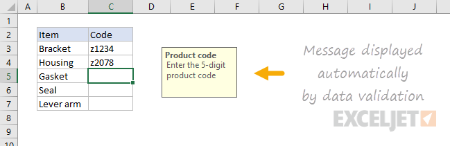
Data validation is a feature in Excel used to control what a user can enter into a cell. For example, you could use data validation to make sure a value is a number between 1 and 6, make sure a date occurs in the next 30 days, or make sure a text entry is less than 25 characters. When a user enters an invalid value, data validation can display a message telling the user what is allowed, as shown below:
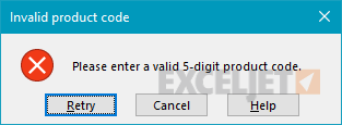
Data validation can also stop invalid user input. For example, if a product code fails validation, you can display a message like this:
In addition, data validation can be used to present the user with a predefined choice in a drop-down menu:

This is a nice way to show a user what options are available and valid.
Data validation controls
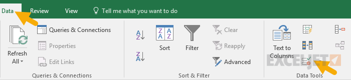
Data validation is implemented via rules defined in Excel's user interface on the Data tab of the ribbon.
Important limitation
It is important to understand that data validation can be easily defeated. If a user copies data from a cell without validation to a cell with data validation, the validation is destroyed (or replaced). Data validation is a good way to let users know what is allowed or expected, but it is not a foolproof way to guarantee input.
Defining data validation rules
Data validation is defined in a window with 3 tabs: Settings, Input Message, and Error Alert:
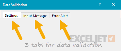
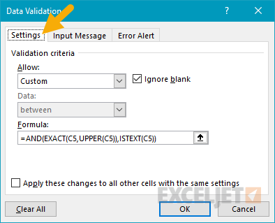
The settings tab is where you enter validation criteria. There are a number of built-in validation rules with various options, or you can select "Custom", and use your own formula to validate input, as seen below:
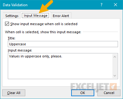
The Input Message tab defines a message to display when a cell with validation rules is selected. This Input Message is completely optional. If no input message is set, no message appears when a user selects a cell with data validation applied. The input message has no effect on what the user can enter — it simply displays a message to let the user know what is allowed or expected.
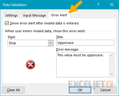
The Error Alert Tab controls how validation is enforced. For example, when the Style is set to "Stop", invalid data triggers a window with a message, and the input is not allowed.
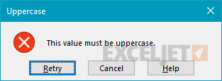
The user sees a message like this:
When style is set to Information or Warning, a different icon is displayed with a custom message, but the user can ignore the message and enter values that don't pass validation. The table below summarizes behavior for each error alert option.
| Alert Style | Behavior |
|---|---|
| Stop | Stops users from entering invalid data in a cell. Users can retry, but must enter a value that passes data validation. The Stop alert window has two options: Retry and Cancel. |
| Warning | Warns users that data is invalid. The warning does nothing to stop invalid data. The Warning alert window has three options: Yes (to accept invalid data), No (to edit invalid data) and Cancel (to remove the invalid data). |
| Information | Informs users that data is invalid. This message does nothing to stop invalid data. The Information alert window has 2 options: OK to accept invalid data, and Cancel to remove it. |
Data validation options
When a data validation rule is created, there are eight options available to validate user input:
Any Value - no validation is performed. Note: if data validation was previously applied with a set Input Message, the message will still display when the cell is selected, even when Any Value is selected.
Whole Number - only whole numbers are allowed. Once the whole number option is selected, other options become available to further limit input. For example, you can require a whole number between 1 and 10.
Decimal - works like the whole number option, but allows decimal values. For example, with the Decimal option configured to allow values between 0 and 3, values like 0.5, 1.5, 2, and 2.75 are all allowed.
List - only values from a predefined list are allowed. The values are presented to the user as a drop-down menu control. Allowed values can be hardcoded directly into the Settings tab or specified as a range on the worksheet.
Date - only dates are allowed. For example, you can require a date between January 1, 2018, and December 31, 2021, or a date after June 1, 2018.
Time - only times are allowed. For example, you can require a time between 9:00 AM and 5:00 PM, or only allow times after 12:00 PM.
Text length - validates input based on the number of characters or digits. For example, you could require code that contains 5 digits.
Custom - validates user input using a custom formula. In other words, you can write your own formula to validate input. Custom formulas greatly extend the options for data validation. For example, you could use a formula to ensure a value is uppercase, a value contains "xyz", or a date is a weekday in the next 45 days.
Ignore blank - tells Excel not to validate cells that contain no value. In practice, this setting seems to affect only the command "circle invalid data". When enabled, blank cells are not circled even if they fail validation.
Apply these changes to other cells with the same settings - this setting will update the validation applied to other cells when it matches the (original) validation of the cell(s) being edited.
Note: You can also manually select all cells with data validation applied using Go To + Special, as explained below.
Simple drop-down menu
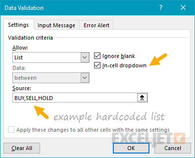
You can provide a dropdown menu of options by hardcoding values into the settings box or selecting a range on the worksheet. For example, to restrict entries to the actions "BUY", "HOLD", or "SELL", you can enter these values separated with commas as seen below:
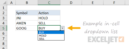
When applied to a cell in the worksheet, the dropdown menu works like this:
Another way to supply values to a dropdown menu is to use a worksheet reference. For example, with sizes (i.e., small, medium, etc.) in the range F3:F6, you can supply this range directly inside the data validation settings window:
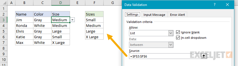
Note that the range is entered as an absolute address to prevent it from changing as the data validation is applied to other cells.
Tip: Click the small arrow icon at the far right of the source field to make a selection directly on the worksheet so you don't have to enter the range manually.
You can also use named ranges to specify values. For example, with the named range called "sizes" for F3:F7, you can enter the name directly in the window, starting with an equal sign:
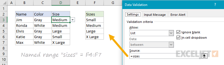
Named ranges are automatically absolute, so they won't change as the data validation is applied to different cells. If named ranges are new to you, this page has a good overview and a number of related tips.
You can also create dependent dropdown lists with a custom formula.
Tip - if you use an Excel Table for dropdown values, Excel will expand or contract the table automatically when dropdown values are added or removed. In other words, Excel will automatically keep the dropdown in sync with values in the table as values are changed, added, or removed. If you're new to Excel Tables, you can see a demo in this video on Table shortcuts.
Data validation with a custom formula
Data validation formulas must be logical formulas that return TRUE when input is valid and FALSE when input is invalid. For example, to require numeric input in cell A1, you could use the ISNUMBER function in a formula like this:
=ISNUMBER(A1)
If a user enters a value like 10 in A1, ISNUMBER returns TRUE, and data validation succeeds. If they enter a value like "apple" in A1, ISNUMBER returns FALSE, and data validation fails. To enable data validation with a formula, select "Custom" in the settings tab, then enter a formula in the formula bar beginning with an equal sign (=) as usual.
Troubleshooting formulas
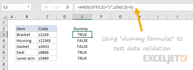
Excel ignores data validation formulas that return errors. If a formula isn't working, and you can't figure out why, set up dummy formulas to make sure the formula is performing as you expect. Dummy formulas are simply data validation formulas entered directly on the worksheet so that you can see what they return easily. The screen below shows an example:
Once you get the dummy formula working as you want, simply copy and paste it into the data validation formula area.
If this dummy formula idea is confusing to you, watch this video, which shows how to use dummy formulas to perfect conditional formatting formulas. The concept is exactly the same.
Data validation formula examples
The possibilities for data validation custom formulas are virtually unlimited. To allow only 5-character values that begin with "z", you could use:
=AND(LEFT(A1)="z",LEN(A1)=5)
This formula returns TRUE only when a code is 5 digits long and starts with "z". To allow only a date within 30 days of today:
=AND(A1>TODAY(),A1<=(TODAY()+30))
To allow only unique values:
=COUNTIF(range,A1)<2
To allow only an email address
=ISNUMBER(FIND("@",A1)
Data validation to circle invalid entries
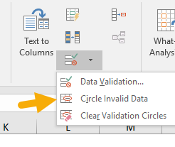
Once data validation is applied, you can ask Excel to circle previously entered invalid values. On the Data tab of the ribbon, click Data Validation and select "Circle Invalid Data":
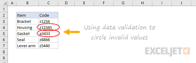
For example, the screen below shows values circled that fail validation with this custom formula:
=AND(LEFT(A1)="z",LEN(A1)=5)
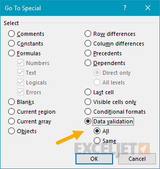
Find cells with data validation
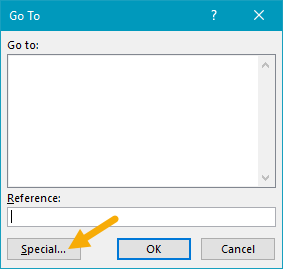
To find cells with data validation applied, you can use the Go To > Special dialog. Type the keyboard shortcut Control + G, then click the Special button. When the Dialog appears, select "Data Validation":
Copy data validation from one cell to another
To copy validation from one cell to other cells. Copy the cell(s) normally that contain the data validation you want, then use Paste Special + Validation. Once the dialog appears, type "n" to select validation, or click validation with the mouse.
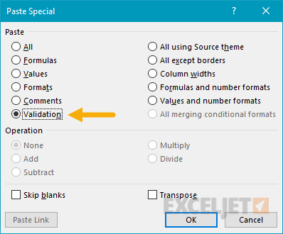
Note: You can use the keyboard shortcut Control + Alt + V to invoke Paste Special without the mouse.
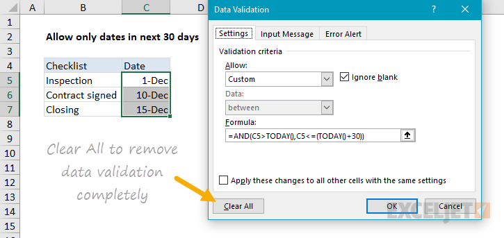
Clear all data validation
To clear all data validation from a range of cells, make the selection, then click the Data Validation button on the Data tab of the ribbon. Then click the "Clear All" button:
To clear all data validation from a worksheet, select the entire worksheet, then follow the same steps above.


