Summary
Excel Tables have a boring (and confusingly generic) name, but they are packed with useful features. This article is a summary of the things you should know about Excel Tables.
Excel Tables are one of the most interesting and useful features in Excel. If you need a range that expands to include new data, and if you want to refer to data by name instead of by address, Excel Tables are for you. This article provides an introduction and overview.
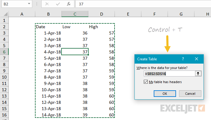
1. Creating a table is fast
You can create an Excel Table in less than 10 seconds. First, remove blank rows and make sure all columns have a unique name, then put the cursor anywhere in the data and use the keyboard shortcut Control + T. When you click OK, Excel will create the table.
2. Navigate directly to tables
Like named ranges, tables will appear in the namebox dropdown menu. Just click the menu, and select the table. Excel will navigate to the table, even if it's on a different tab in a workbook.
3. Tables provide special shortcuts
When you convert regular data to an Excel Table, almost every shortcut you know works better. For example, you can select rows with shift + space, and columns with control + space. These shortcuts make selections that run precisely to the edge of the table, even when you can't see the edge of the table. Watch the video below for a quick rundown. See also: The Excel shortcuts you really should know
Video: Shortcuts for Excel tables
4. Painless drag and drop
Tables make it much easier to rearrange data with drag and drop. After you've selected a table row or column, simply drag to a new location. Excel will quietly insert the selection at the new location, without complaining about overwriting data.
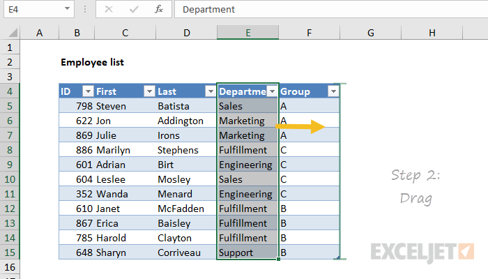
Note: you must select the entire row or column. For columns, that includes the header.
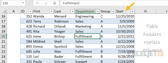
5. Table headers stay visible
One frustration when working with a large set of data is that table headers disappear as you scroll down the table. Tables solve this problem in a clever way. When column headers scroll off the top of the table, Excel silently replaces worksheet columns with table headers.
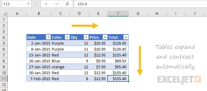
6. Tables expand automatically
When new rows or columns are added to an Excel Table, the table expands to enclose them. In a similar way, a table automatically contracts when rows or columns are deleted. When combined with structured references (see below), this gives you a dynamic range to use with formulas.
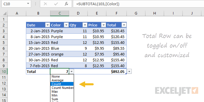
7. Totals without formulas
All tables can display an optional Total Row. The Total Row can be easily configured to perform operations like SUM and COUNT without entering a formula. When the table is filtered, these totals will automatically calculate on visible rows only. You can toggle the Total Row on and off with the shortcut control + shift + T.
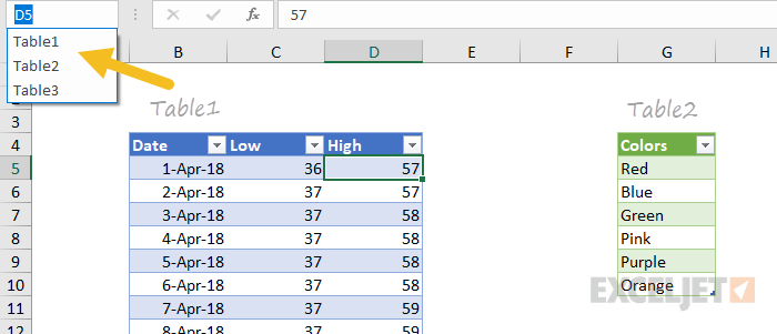
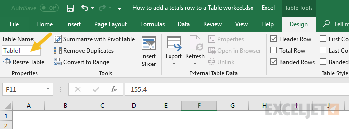
8. Rename a table anytime
All tables are automatically assigned a generic name like Table1, Table2, etc. However, you can rename a table at any time. Select any cell in the table and enter a new name in the Table Tools menu.
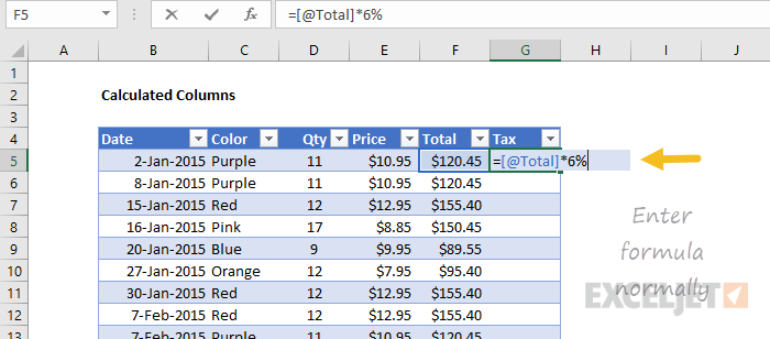
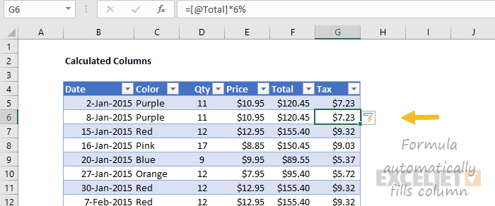
9. Fill formulas automatically
Tables have a feature called calculated columns that makes entering and maintaining formulas easier and more accurate. When you enter a standard formula in a column, the formula is automatically copied throughout the column, with no need for copy and paste.
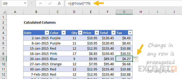
10. Change formulas automatically
The same feature also handles formula changes. If you make a change to the formula anywhere in a calculated column, the formula is updated throughout the entire column. In the screen below, the tax rate has been changed to 7% in one step.
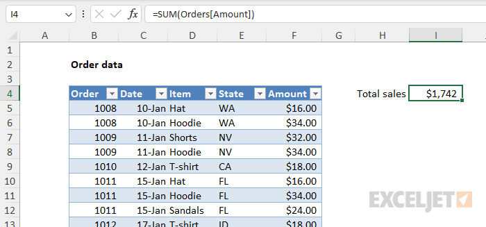
11. Human-readable formulas
Tables use a special formula syntax to refer to parts of a table by name. This feature is called "structured references". For example, to SUM a column called "Amount" in a table called "Orders", you can use a formula like this:
=SUM(Orders[Amount])
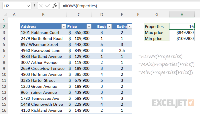
12. Easy dynamic ranges
The single biggest benefit of tables is that they automatically expand as new data is added, creating a dynamic range. You can easily use this dynamic range in your formulas. For example, the table in the screen below is named "Properties". The following formulas will always return correct values, even as data is added to the table:
=ROWS(Properties)
=MAX(Properties[Price])
=MIN(Properties[Price])
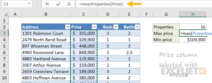
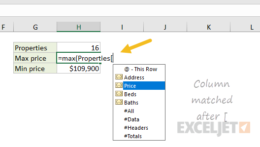
13. Enter structured references with the mouse
An easy way to enter structured references in formulas is to use the mouse to select part of the table. Excel will automatically enter the structured reference for you. In the screen below, the price column was selected after entering =MAX(
14. Enter structured references by typing
Another way to enter structured references is by typing. When you type the first few letters of a table in a formula, Excel will list matching table names below.
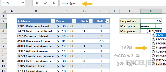
Use the arrow keys to select and the TAB key to confirm. To enter a column name, enter an opening square bracket [ after the table name, follow the same process: type a few letters, select with arrow keys, and use TAB to confirm.
Video: Introduction to Structured References and Tables
15. Check structured references with a formula
You can quickly check a structured reference with the formula bar. For example, the following formula will select data in the "Address" column in the "Properties" table shown above:
=Properties[Address]
And this formula will select the headers of the table:
=Properties[#Headers]
Video: How to query a table with formulas
Video: How to use SUMIFS with a table
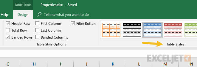
16. Change table formatting with one click
All Excel tables have a style applied by default, but you can change this at any time. Select any cell in the table and use the Table Styles menu on the Table Tools tab of the ribbon. With one click, the table will inherit the new style.
17. Remove all formatting
Table formatting is not a requirement of Excel tables. To use a table without formatting, select the first style in the styles menu, which is called "None".
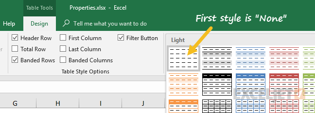
Tip: You can use this style to remove all table formatting before converting a table back to a normal range.
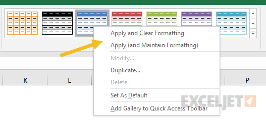
18. Override local formatting
When you apply a table style, local formatting is preserved by default. However, you can optionally override local formatting if you want. Right-click any style and choose "Apply and Clear formatting":
19. Set a default table style
You can right-click any style and choose "Set as Default". New tables in the same workbook will now use the default you set.
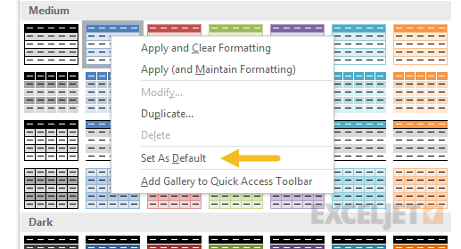
Note: To set a default table style in new workbooks, create a custom start-up template as described in this article. In the template file, set the default table style of your choice.
20. Use a Table with a pivot table
When you use a table as the source for a pivot table, the pivot table will automatically stay up to date with changes in data. Watch the video below to see how this works.
Video: Use a table for your next pivot table
21. Use a table to create a dynamic chart
Tables are a great way to create dynamic charts. New data in the table will automatically appear in the chart, and charts will exclude filtered rows by default.
Video: How to build a simple dynamic chart
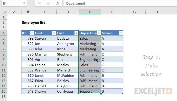
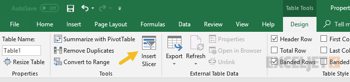
22. Add a slicer to a table
Although all tables get filter controls by default, you can also add a slicer to a table to make it easy to filter data with large buttons. To add a slicer to a table, click the Insert Slicer button on the Design tab of the Table Tools menu.
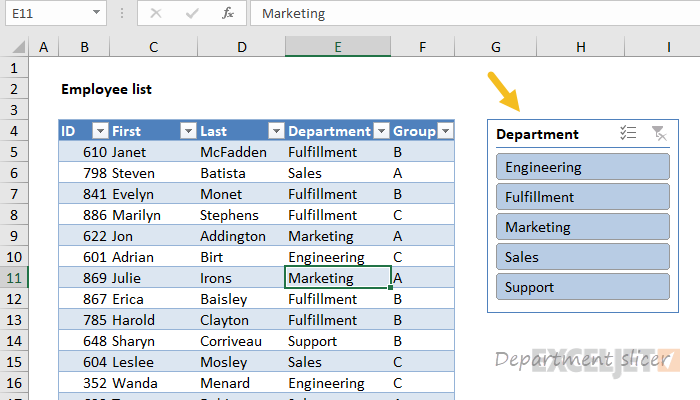
The table below has a slicer for Department:
23. Get rid of a table
To get rid of a table, use the Convert to Range command on the Table Tools tab of the ribbon.
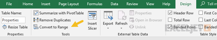
You might be surprised to see that converting a table back to a normal range doesn't remove formatting. To remove table formatting, first apply the "None" table style, then use "Convert to Range".


