
Summary
A curated guide to the most useful Excel shortcuts for Windows and Mac, with explanations, tips, and videos. Covers navigation, selection, data entry, formatting, formulas, and more.
A lot of your time in Excel is spent on very repetitive actions. The good news is that Excel has hundreds of keyboard shortcuts that can help speed these tasks up. The bad news is that there are so many shortcuts, it's easy to get confused about which ones to use. This article focuses on the shortcuts I think most Excel users should know. These are time-saving shortcuts you can use day after day.
There are over 200 Excel shortcuts. This article explains the ones I think are most useful. – Dave
Table of contents
NAVIGATION
Next worksheet / Previous worksheet
Often, you'll need to switch back and forth between different worksheets in the same workbook. If you are working in a large workbook with many sheets, this can be annoying with a mouse, because some sheets may not be visible. However, with the shortcuts below, you can quickly move forward and backward through sheets in a workbook using only the keyboard.
| Shortcut | Win | Mac |
|---|---|---|
| Move to the next worksheet | Ctrl PgDn | ⌥ → |
| Move to the previous worksheet | Ctrl PgUp | ⌥ ← |
Video: Shortcuts to navigate worksheets
Next workbook / Previous workbook
Another common task in Excel is switching between open workbooks. Perhaps you are switching between workbooks to see what's changed, or maybe you are copying values from one workbook into another. The fastest way to switch workbooks in Excel is to use these shortcuts:
| Shortcut | Win | Mac |
|---|---|---|
| Move to the next workbook | Ctrl Tab | ⌘ ` |
| Move to the previous workbook | Ctrl Shift Tab | ⌘ ⇧ ` |
In Windows, you can also use Ctrl + F6 and Ctrl + Shift + F6 to move to the next and previous workbook.
On a Mac, the shortcut for cycling between open windows in an application is Command + `. (See also: Excel shortcuts on the Mac.) This is the back-tick or grave accent key, which is usually found above the Tab key. Note this is a system-level shortcut, and not specific to Excel. If you have trouble, check System Settings > Keyboard > Keyboard Shortcuts to confirm that "Move focus to the next window" is enabled.
Video: Shortcuts to navigate workbooks
Expand or collapse ribbon
At first glance, this might seem like a minor convenience. But here's the thing: that ribbon is hogging 4 precious rows of screen real estate, even when you're completely ignoring it. If you're working on a laptop, you want every row you can get. The good news is you can banish the ribbon with a quick keystroke, and summon it when needed. Give your spreadsheet room to breathe.
| Shortcut | Win | Mac |
|---|---|---|
| Expand or collapse ribbon | Ctrl F1 | ⌘ ⌥ R |
Move to edge of data region
This shortcut sounds boring, but don't let that fool you. It's vital if you work with big lists or tables. Why? Because scrolling is a huge waste of time. Instead of manually dragging your way through endless rows and columns like you're on some kind of digital treadmill, just drop your cursor into the data and hit Control + Arrow key. Boom. You'll teleport instantly to the edge of your data range in whatever direction you choose.
Here's how it works: the cursor zips along until it hits the first empty cell, or the edge of the spreadsheet, whichever comes first. Starting in an empty cell? The behavior flips: now the cursor hunts down the first cell with actual content and parks there. Once you understand how this works, you'll find these shortcuts addictive.
| Shortcut | Win | Mac |
|---|---|---|
| Move to right edge of data region | Ctrl → | ⌘ → |
| Move to left edge of data region | Ctrl ← | ⌘ ← |
| Move to top edge of data region | Ctrl ↑ | ⌘ ↑ |
| Move to bottom edge of data region | Ctrl ↓ | ⌘ ↓ |
Mac users: Command or Control both work. Excel doesn't care.
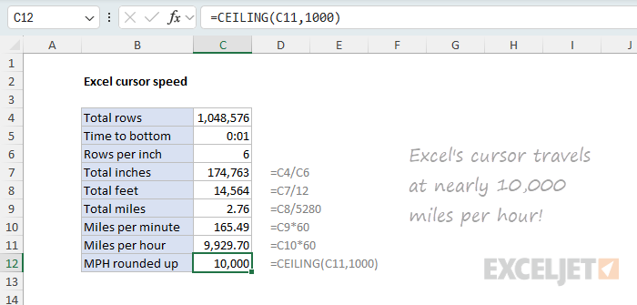
Excel's speedy cursor. Modern Excel has 1,048,576 rows. Drop your cursor in A1, hit Control + down arrow, and you'll hit the bottom in under a second. Quick napkin math: at roughly 6 rows per inch, that's 1,048,576 ÷ 6 = 174,763 inches. Divide by 12 for feet (14,564), then by 5,280 for miles, and we get about 2.76 miles. Moving at 2.76 a second works out to 165.6 miles per minute, which scales up to 9,936 miles per hour. In other words, your cursor is basically traveling at 10,000 mph. That's faster than a speeding bullet. You'll never beat the cursor scrolling. Ever.
Extend selection to the edge of data
Navigating at high speed through a large table is great fun, but what really makes this idea powerful is selecting huge swaths of cells at the same time. Because when you try to select large collections of cells manually (let's say 10,000 rows), you will be scrolling a long time. A really long time.
To save your sanity and avoid all that scrolling, just add the Shift key to the Control + Arrow shortcut, and you will extend the current selection to include all the cells along the way. The best part about using Shift + Control + Arrow is that your selection will be perfectly accurate. Even though the cursor is moving incredibly fast, it will stop on a dime at the edge of a data region.
| Shortcut | Win | Mac |
|---|---|---|
| Extend selection to right edge of data | Ctrl Shift → | ⌘ ⇧ → |
| Extend selection to left edge of data | Ctrl Shift ← | ⌘ ⇧ ← |
| Extend selection to top edge of data | Ctrl Shift ↑ | ⌘ ⇧ ↑ |
| Extend selection to bottom edge of data | Ctrl Shift ↓ | ⌘ ⇧ ↓ |
Video: Shortcuts for extending selections
Move to first cell in worksheet
Getting around larger worksheets can get really tedious. Sure, you can use the scroll bars to scroll the worksheet into position, but scroll bars require control and patience. If you just want to get back to the first screen in a worksheet, use the shortcut below. This will bring you straight back to cell A1, no matter how far you've wandered.
| Shortcut | Win | Mac |
|---|---|---|
| Move to first cell in worksheet | Ctrl Home | Fn ⌃ ← |
Move to last cell in worksheet
In a similar way, you can jump to the "last cell" in a worksheet using the shortcut below. What is the last cell? Good question. The last cell in a worksheet is at the intersection of the last row that contains data and the last column that contains data. Often, the last cell in a worksheet doesn't contain any data itself. It just defines the lower right edge of a rectangle that makes up the used range of the worksheet.
| Shortcut | Win | Mac |
|---|---|---|
| Move to last cell in worksheet | Ctrl End | Fn ⌃ → |
One good use of this shortcut is to check for stray data. You can use this to make sure you don't accidentally print 16 blank pages because there's a random "x" in cell Z1234. It's also useful when you notice that a workbook is suddenly a lot bigger on disk than it should be. In this case, it's likely that there's extra data somewhere in the worksheet.
SELECTING
Select all
Most people know Control + A as the "select all" shortcut, but it's smarter than you think. Its behavior changes based on context. When the cursor sits in an empty cell, Control + A selects the entire worksheet. But place that cursor inside a group of cells that contain data, and Control + A selects only that group instead.
The behavior changes again when the cursor is in an Excel Table. The first time you use Control + A, the table data is selected. The second time, both the table data + table header are selected. Finally, the third time you use Control + A, the entire worksheet is selected.
| Shortcut | Win | Mac |
|---|---|---|
| Select all | Ctrl A | ⌘ A |
Select current region
This shortcut selects the contiguous block of data surrounding the active cell. Unlike Control + A, which behaves differently depending on context, this shortcut always selects the current region and nothing more. It's a reliable way to grab a block of data when you're not sure exactly how far it extends. Especially useful before copying, formatting, or creating a chart.
| Shortcut | Win | Mac |
|---|---|---|
| Select current region | Ctrl Shift * | ⌘ ⇧ * |
Select row / select column
Both rows and columns can be selected with keyboard shortcuts. To select a row, use Shift + Space. To select a column, use Control + Space. Once you have a row or column selected, you can hold down the shift key and extend your selection by using the appropriate arrow keys. For example, if the cursor is in row 10 and you press Shift + Space, row 10 will be selected. You can then hold the shift key down and use the Up or Down arrow keys to select additional rows above or below row 10.
Once you have specific rows or columns selected, you can use other keyboard shortcuts to insert, delete, hide, and unhide rows and columns.
| Shortcut | Win | Mac |
|---|---|---|
| Select row | Shift Space | ⇧ Space |
| Select column | Ctrl Space | ⌃ Space |
If you are working in an Excel table, these same shortcuts will select rows and columns within the table, not the entire worksheet.
Video: Shortcuts for selecting cells
Select non-adjacent cells
Sometimes you need to select cells that are scattered across your worksheet. Maybe you want to format them all at once, enter the same data everywhere (hello, Control + Enter!), or just use the status bar to peek at a quick SUM of your random collection. Whatever the reason, this shortcut is your bridge between cells. Select your first cell (or group of cells), then hold down Control (or Command on Mac) and click away. Each click adds another cell to your growing collection of selections.
| Shortcut | Win | Mac |
|---|---|---|
| Add cells to selection | Ctrl Click | ⌘ Click |
Select visible cells only
Here's a shortcut that solves a problem you might not even know you have. When you copy a range that contains hidden rows or columns, Excel copies the hidden cells too. This can wreak havoc when you paste, because suddenly you've got data you can't even see mixed in with data you intended to copy. The fix? Select your range, then use this shortcut to trim the selection down to only the cells you can actually see. Now when you copy and paste, you get exactly what you expected.
| Shortcut | Win | Mac |
|---|---|---|
| Select visible cells only | Alt ; | ⌘ ⇧ Z |
Show the active cell on worksheet
Ever lose your cursor in a large worksheet? Sure, you could tap an arrow key to summon it back (but then you've moved to a new cell, oops). Or you could play detective with the name box. But why do any of that when you can use the shortcut below? It's like a "find my cursor" beacon that instantly scrolls your active cell into view, perfectly centered and ready for action.
| Shortcut | Win | Mac |
|---|---|---|
| Show active cell | Ctrl Backspace | ⌘ Delete |
Video: Shortcuts to move the active cell
Find next match
Rather basic, but worth knowing: once you've set up a find, and have found at least one match, you can keep finding "the next match" with the shortcut below. This is a nice way to step through matches in a worksheet methodically. The first shortcut below opens the Find dialog box. The second shortcut finds the next match.
| Shortcut | Win | Mac |
|---|---|---|
| Find | Ctrl F | ⌘ F |
| Find next match | Shift F4 | ⌘ G |
By the way, on Windows and Mac, you can also use Control + H to activate "Find and Replace".
Video: Shortcuts to find and replace
Display 'Go To' dialog box
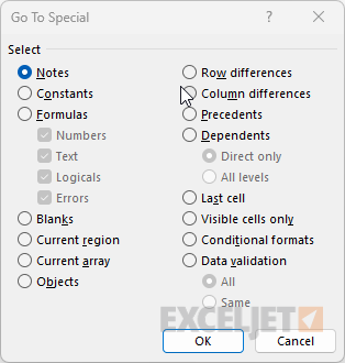
The Go To Special dialog is a bit like the Paste Special Dialog. Within lies a treasure trove of utility hidden by a boring-sounding name. Did you know you can use Go To Special to select only formulas? Only constants? Only blank cells? Cells that have data validation applied? You can do all that and a lot more. Unfortunately, the shortcut below only gets you halfway there, to the "Go To" dialog box. Then you need to click the Special button to get all the way to Go To Special.
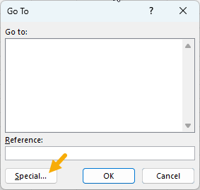
Still a worthy shortcut, however, because Go To Special is a gateway to many tricky and powerful features. See the videos below for examples.
| Shortcut | Win | Mac |
|---|---|---|
| Display Go To dialog box | Ctrl G | Fn ⌃ G |
Videos on Go To Special:
- Shortcuts for Go To Special
- Go To Special to delete blank rows
- Go To Special to weed out rows that are missing values
ENTERING DATA
Start a new line in the same cell
This is not so much a shortcut as something you simply must know to enter multiple lines in a single cell. This is often a puzzle to Excel users (for obvious reasons) and I have no doubt that it has resulted in millions of Google searches. Here is the answer revealed:
| Shortcut | Win | Mac |
|---|---|---|
| Start new line in same cell | Alt Enter | ⌃ ⌥ Return |
Enter the same value in multiple cells
This shortcut may not seem interesting, but you'll be surprised how often you use it once you understand how it works. Use Control + Enter when you want to enter the same value in multiple cells at once. This is a great way to save keystrokes when you want to enter the same value in a group of cells, even a group of non-contiguous cells. (See the previous shortcut for selecting non-adjacent cells.)
| Shortcut | Win | Mac |
|---|---|---|
| Enter same data in multiple cells | Ctrl Enter | ⌘ Return |
By the way, Control + Enter also has another handy feature: use it when you want to enter a value and remain in the same cell after hitting return.
Video: Shortcut for entering data in more than one cell
Insert current date / Insert current time
No Excel shortcut guide would be complete without mentioning these classics for the current date and time.
| Shortcut | Win | Mac |
|---|---|---|
| Insert current date | Ctrl ; | ⌃ ; |
| Insert current time | Ctrl Shift : | ⌘ ; |
To enter a date and time in a single cell, insert the current date, then a space, then insert the current time. Note that Excel will enter the current date or time using a valid Excel date in serial number format, with dates as integers and times as decimal values. You can then apply date or time formatting as you like.
Note: these shortcuts create static values that will not change. If you want to enter a date or time that will update automatically, use the TODAY or NOW functions.
Video: Shortcuts for the current date and time in Excel
Fill down / Fill right
Do you enjoy copying and pasting values in Excel? If so, ignore these shortcuts! Otherwise, these gems allow you to quickly copy data from one cell to another in one step, without using copy and paste. These shortcuts are very satisfying when they fit the data you are wrangling.
| Shortcut | Win | Mac |
|---|---|---|
| Fill down | Ctrl D | ⌘ D |
| Fill right | Ctrl R | ⌘ R |
You can use these same shortcuts to copy data to multiple cells, too. The trick is to select both the source cells and target cells before you use the shortcut. For example, to copy values from the row above into the next 6 rows in a table, select the source row and the next 6 target rows, then use Control + D.
Video: Shortcuts to enter data
Flash fill
Flash Fill is a modern Excel feature that deserves a spot on this list. It recognizes patterns in your data and fills in values automatically. Type an example or two of what you want in a column adjacent to your data, then use this shortcut. Excel will analyze the pattern and fill the remaining cells in one shot. It works for extracting text, combining values, reformatting data, and all sorts of other transformations you'd normally need formulas for.
| Shortcut | Win | Mac |
|---|---|---|
| Flash fill | Ctrl E | ⌘ E |
Note: A working formula is always more reliable and repeatable than Flash Fill, but getting a formula working can take time. Plus, you will probably want to convert the results to values, which is another step. When Flash Fill works, it is very handy.
EDITING
Edit the active cell
You can either double-click a cell or use F2 (Mac: Control + U) to enter "edit mode" for the active cell. This is the starting point for changing a cell's contents without erasing what's already there.
| Shortcut | Win | Mac |
|---|---|---|
| Edit active cell | F2 | ⌃ U |
You can always edit the text or formula in a selected cell with the formula bar; no action needed.
Video: Shortcuts for editing cells
Display the Paste Special dialog box
There are so many things you can do with paste special; it's a topic in itself. At the very least, you probably already use paste special to strip out unwanted formatting and formulas (Paste Special > Values). But did you know that you can also paste formatting, paste column widths, multiply and add values in place, and even transpose tables? Yep, it's all there.
Using Paste Special is a four-step process:
- Copy the data you want to work with.
- Open the Paste Special dialog box.
- Choose the operation(s) you want to perform.
- Click OK to apply the operation(s).
The shortcut below opens the Paste Special dialog box:
| Shortcut | Win | Mac |
|---|---|---|
| Display the Paste Special dialog box | Ctrl Alt V | ⌘ ⌃ V |
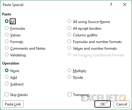
Once the Paste Special dialog box is open, you can select the operation you want to perform by typing a letter as shown in the table below:
| Operation | Key |
|---|---|
| Paste Special > All | a |
| Paste Special > Formulas | f |
| Paste Special > Values | v |
| Paste Special > Formats | t |
| Paste Special > Comments and Notes | c |
| Paste Special > All using source theme | h |
| Paste Special > All except borders | x |
| Paste Special > Column widths | w |
| Paste Special > Formulas and number formats | r |
| Paste Special > Values and number formats | u |
| Paste Special > All merging conditional formats | g |
| Paste Special > None | o |
| Paste Special > Add | d |
| Paste Special > Subtract | s |
| Paste Special > Multiply | m |
| Paste Special > Divide | i |
| Paste Special > Skip blanks | b |
| Paste Special > Transpose | e |
Paste values in one step
In 2025, Excel 365 introduced a dedicated shortcut to paste values: Ctrl + Shift + V. This shortcut is equivalent to the Paste Special > Values operation.
| Shortcut | Win | Mac |
|---|---|---|
| Paste values | Ctrl Shift V | ⌘ ⇧ V |
Toggle autofilter
Using Excel's filters? Remember this shortcut. On the surface, it's simple: one keystroke toggles filters on and off. But here's the clever bit: turning off the autofilter also wipes out any active filters. Translation? If you've got filters stacked on filters and just want to start fresh, hit the shortcut twice: once to nuke everything, once to bring back a clean slate. It's like an "undo all filters" button that Excel forgot to include. Way faster than clicking through dropdown menus like some kind of medieval peasant*.
| Shortcut | Win | Mac |
|---|---|---|
| Toggle Autofilter | Ctrl Shift L | ⌘ ⇧ F |
** To be clear, medieval peasants did not have drop-down menus to worry about.*
Insert table
If you're not using Excel Tables, you should be. Tables give you structured references, dynamic ranges, automatic formatting, built-in filters, and easy totals. And the fastest way to create one is with this shortcut. Select any cell in your data and press Control + T. Excel will detect the range, ask you to confirm, and convert your data into a proper table. Once you start using tables, you'll wonder how you ever lived without them.
| Shortcut | Win | Mac |
|---|---|---|
| Insert table | Ctrl T | ⌘ T |
Video: Shortcuts for Excel Tables
Undo / Redo
You probably already use Undo, but it's worth remembering that Excel supports multiple levels of undo, up to 100 steps in most versions. That means you can walk back through a long chain of changes if something goes sideways. Redo is equally useful: it lets you reapply any action you just undid. Together, they let you experiment freely. Remember that some actions in Excel (like deleting a sheet) have no undo.
| Shortcut | Win | Mac |
|---|---|---|
| Undo | Ctrl Z | ⌘ Z |
| Redo | Ctrl Y | ⌘ Y |
Repeat last action
This shortcut is deceptively powerful. Outside of edit mode, F4 repeats whatever action you just performed. Applied bold formatting? F4 does it again. Inserted a row? F4 inserts another. Deleted a column? F4 deletes the next one. It works with formatting, inserting, deleting, and many other operations. It's like a one-key macro for your last action, and once you start using it, you'll reach for it constantly.
| Shortcut | Win | Mac |
|---|---|---|
| Repeat last action | F4 | ⌘ Y |
Note: F4 does double duty. When you're editing a formula, it toggles cell references between absolute and relative. Outside of edit mode, it repeats your last action. Context is everything.
Drag and drop
Drag and drop in Excel is more capable than most people realize. A plain drag cuts and moves cells to a new location. But add modifier keys, and you unlock a whole family of operations: copy, insert, insert a copy, or even move cells to a different worksheet. These are mouse shortcuts, not keyboard shortcuts, but they're too useful to ignore.
| Shortcut | Win | Mac |
|---|---|---|
| Drag and cut (move) | Drag | Drag |
| Drag and copy | Ctrl Drag | ⌥ Drag |
| Drag and insert | Shift Drag | ⇧ Drag |
| Drag and insert copy | Ctrl Shift Drag | ⌥ ⇧ Drag |
Drag and insert is particularly handy for moving rows and columns around without messing up other data. However, it's a slippery shortcut that takes some practice...try it!
Video: Shortcuts for drag and drop
FORMATTING
Format Cells dialog box
This shortcut is a gateway to many formatting options. When regular cells are selected, it displays the Format Cells dialog box with the last tab used automatically selected. This is a very fast way to access fonts, borders, fills, alignment, and number formats no matter where you are in Excel, and even when the ribbon is collapsed.
| Shortcut | Win | Mac |
|---|---|---|
| Display Format Cells dialog | Ctrl 1 | ⌘ 1 |
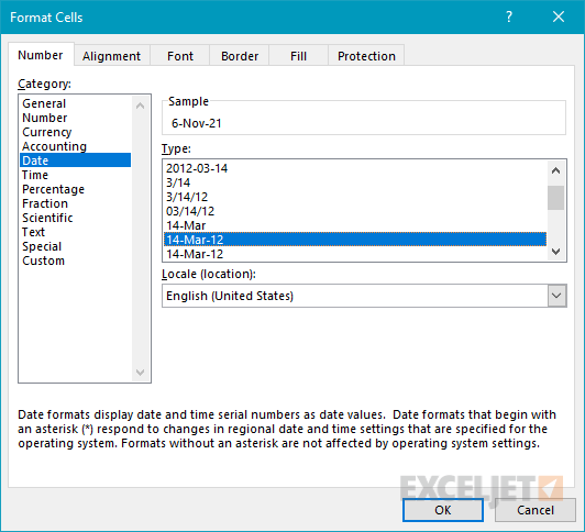
When you're working with a chart, the same shortcut will open various formatting dialogs, depending on what you have selected. For example, if you have the chart area selected, it will open the Format Chart Area dialog. If you have data bars selected, it will open the Format Data Series dialog, and so on. You can also use this shortcut when working with shapes and SmartArt.
Note: Special thanks to Excel charts guru Jon Peltier for pointing out to me many years ago that Control + 1 is not just for formatting cells!
Give this shortcut a try before you hunt down a formatting option in the ribbon. It's a fast way to get to many formatting options, and it works even when the ribbon is collapsed.
Video: Shortcuts for formatting
Bold, italic, underline
Boring, yet essential shortcuts for bold, italic, and underline.
| Shortcut | Win | Mac |
|---|---|---|
| Bold | Ctrl B | ⌘ B |
| Italic | Ctrl I | ⌘ I |
| Underline | Ctrl U | ⌘ U |
You can also use these shortcuts to format specific words and characters. Just double click the cell to enter edit mode, select the text you want to format, and use these shortcuts.
Strikethrough
This one makes the list because it's surprisingly hard to find. Strikethrough isn't on the ribbon by default, so you either have to dig through the Format Cells dialog or know the shortcut. And a lot of people need it for crossing off completed items, marking data as obsolete, or just visually flagging something without deleting it.
| Shortcut | Win | Mac |
|---|---|---|
| Strikethrough | Ctrl 5 | ⌘ ⇧ X |
Number formats
Numbers are the foundation of Excel, and how they appear is controlled by number formats. The shortcuts below let you quickly apply seven common number formats without touching the ribbon.
| Shortcut | Win | Mac |
|---|---|---|
| General format | Ctrl Shift ~ | ⌃ ⇧ ~ |
| Currency format | Ctrl Shift $ | ⌃ ⇧ $ |
| Percentage format | Ctrl Shift % | ⌃ ⇧ % |
| Scientific format | Ctrl Shift ^ | ⌃ ⇧ ^ |
| Date format | Ctrl Shift # | ⌃ ⇧ # |
| Time format | Ctrl Shift @ | ⌃ ⇧ @ |
| Number format | Ctrl Shift ! | ⌃ ⇧ ! |
Each shortcut follows the same pattern: Control + Shift + [symbol]. With a bit of practice, you'll get the idea quickly. Note that "Accounting format" is conspicuously absent.
Video: Shortcuts for number formats
FORMULAS
Toggle absolute/relative reference
If you work regularly with formulas and cell addresses, this shortcut will save you a lot of tedious editing. To use the shortcut, position the cursor in or next to a cell reference you want to change. Then press F4 (Mac: Command + T). Each time you apply the shortcut, Excel will "rotate" one step through relative and absolute options. Starting with a relative reference, the rotation order works like this: absolute, row locked, column locked, relative. So, for example, for the reference A1, you'll see: $A$1, A$1, $A1, and, finally, A1 again.
| Shortcut | Win | Mac |
|---|---|---|
| Toggle absolute and relative references | F4 | ⌘ T |
Autosum selected cells
Autosum works on both rows and columns. Simply select an empty cell to the right or below the cells you want to sum, and type Alt + = (Mac: Command + Shift + T). Excel will guess the range you are trying to sum and insert the SUM function in one step. For more control, first select the range you intend to sum, including the cell where you'd like the SUM function to be. This prevents Excel from guessing wrong about the range in cases where there are blanks or text values in the sum range.
| Shortcut | Win | Mac |
|---|---|---|
| Autosum | Alt = | ⌘ ⇧ T |
For even more satisfaction, you can have Excel insert multiple SUM functions at the same time. To sum multiple columns, select a range of empty cells below the columns. To sum multiple rows, select a range of empty cells in a column to the right of the rows. For the ultimate in shortcut satisfaction, you can have Excel add SUM formulas for an entire table in one step. Select a full table of numbers, including empty cells below the table and to the right of the table. Then use this shortcut:
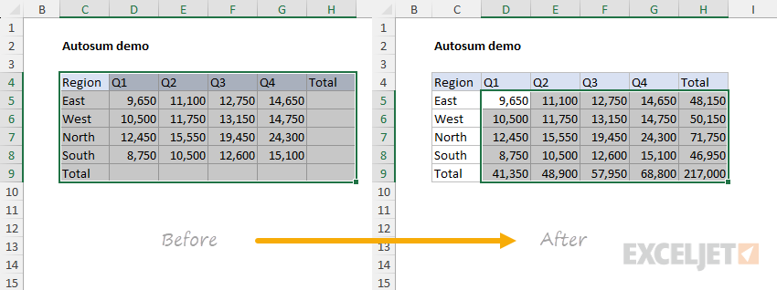
Excel will add a SUM function at the bottom of each column, at the right of each row, and at the lower right corner of the range, giving you column totals, row totals, and a grand total all in one step. In the world of Excel shortcuts, it doesn't get much better than that.
Toggle formulas on and off
It can often be handy to quickly see all the formulas in a worksheet, without clicking into each cell. By using Control + ', you can display all formulas in a worksheet at once. To dismiss the formulas and show the results of the formulas again, type Control + ' a second time.
This gives you a fast way to audit a worksheet. You can see where formulas are used and check for consistency at the same time.
| Shortcut | Win | Mac |
|---|---|---|
| Toggle formulas on and off | Ctrl ' | ⌘ ' |
Video: Shortcuts for formulas
Insert function arguments
This shortcut is a bit of a sleeper. You don't see it mentioned much, but it's pretty cool. What it does: when you're entering a function, after Excel has recognized the function name, typing Control + Shift + A (both platforms) will cause Excel to enter placeholders for all arguments. For example, if you type "=DATE(" and then use Control + Shift + A, Excel gives you "=DATE(year,month,day)". You can then double-click each argument and change it to the address or value you need.
| Shortcut | Win | Mac |
|---|---|---|
| Insert function arguments | Ctrl Shift A | ⌘ ⇧ A |
Video: Shortcuts for functions
Paste name into formula
When you're editing a complex formula, the last thing you need is to leave edit mode to go find the name of a named range or constant. With F3, you don't need to. Just press F3 and Excel will open the named range dialog box so that you can paste in the name you need.
| Shortcut | Win | Mac |
|---|---|---|
| Paste name into formula | F3 |
Video: Shortcuts for named ranges
Accept function with autocomplete
When you're entering a function, Excel will try to guess the name of the function you want, and present an autocomplete list for you to select from. The question is, how do you accept one of the options displayed and yet still stay in edit mode? The trick is to use the tab key. When you press tab, Excel adds any parentheses as needed, then leaves the formula bar active so that you can fill in the arguments as needed. On a Mac, you need to use the down arrow key first to select the function you want, then Tab.
| Shortcut | Win | Mac |
|---|---|---|
| Accept function with autocomplete | Tab | Tab |
WORKING WITH THE GRID
Insert rows / columns
To insert a row or column with a keyboard shortcut, you need to first select an entire row or column, respectively. The shortcut is the same whether you are inserting rows or columns:
- With a laptop keyboard, use Control Shift +.
- With a full keyboard, use Control +
With an entire row selected, this shortcut will insert a row above the selected row. With an entire column selected, this shortcut will insert a column to the left of the selected column.
You can also insert multiple rows and columns. Just select the number of rows or columns you want to insert before using the shortcut.
As already mentioned, you can use a keyboard shortcut to select entire rows or columns: Shift + Space to select a row, Control + Space to select a column.
| Shortcut | Win | Mac |
|---|---|---|
| Insert rows | Ctrl Shift + | ⌘ ⇧ + |
| Insert columns | Ctrl Shift + | ⌘ ⇧ + |
Delete rows / columns
Like inserting rows or columns, the key to deleting rows and columns is to first select an entire row or column. Once you have a row or column selected, the shortcut for deleting rows is the same as for deleting columns: Control + - (both platforms).
With this same shortcut, you can also delete multiple rows and columns. Just select the number of rows or columns you want to delete, then use Control + -.
Note: if you don't have an entire row or column selected when you use Control + -, Excel will present the Delete dialog box, which contains options for deleting rows and columns, and for shifting cells.
| Shortcut | Win | Mac |
|---|---|---|
| Delete rows | Ctrl - | ⌘ - |
| Delete columns | Ctrl - | ⌘ - |
Working with entire rows and columns has benefits.
- Inserting rows and columns is a great way to organize data quickly and safely. By adding an entire row or column, there's no chance you'll accidentally push cells out of alignment somewhere else, because all cells are shifted the same amount.
- In a similar way, deleting columns and rows is a great way to clean up a worksheet quickly. In one fell swoop, you can slice out tons of junk that would be tedious to clean up manually.
Before you start tidying up rows or columns that contain nothing useful, ask yourself: Can I just remove this stuff by deleting rows or columns? If so, then do it! Excel doesn't care how many rows or columns you delete. It will silently replace deleted rows and columns with fresh copies.
Video: Shortcuts to insert and delete rows and columns
Hide and unhide columns
To hide one or more columns, use the shortcut Control + 0 (both platforms). Any columns that intersect the current selection will be hidden. If you prefer, you can also first select entire columns before using this shortcut.
Note that column letters on either side of hidden columns will appear in blue.
To unhide columns, you must first select cells that span either side of the hidden column, or select columns that span the hidden column(s). Then use the keyboard shortcut Control + Shift + 0.
Note that you are just adding Shift to the shortcut for hiding a column.
| Shortcut | Win | Mac |
|---|---|---|
| Hide columns | Ctrl 0 | ⌃ 0 |
| Unhide columns | Ctrl Shift 0 | ⌃ ⇧ 0 |
Hide and unhide rows
To hide one or more rows, use the shortcut Control + 9 (both platforms). Any rows that intersect the current selection will be hidden. You can also first select one or more entire rows if you prefer.
Note that row numbers on either side of hidden rows will appear in blue.
To unhide rows, you must first select rows that span either side of the hidden row, or select entire rows that span the hidden row(s). Then use the keyboard shortcut Control + Shift + 9.
Note that you are just adding Shift to the shortcut for hiding a row.
| Shortcut | Win | Mac |
|---|---|---|
| Hide rows | Ctrl 9 | ⌃ 9 |
| Unhide rows | Ctrl Shift 9 | ⌃ ⇧ 9 |
Video: Shortcuts to hide and unhide rows and columns
CHARTS
Create an embedded chart
To create an embedded chart, first select the data that makes up the chart, including any labels. Then use the keyboard shortcut Alt + F1 (Mac: Fn + Option + F1). Excel will create a new chart on the same worksheet, using your current default chart settings.
| Shortcut | Win | Mac |
|---|---|---|
| Create embedded chart | Alt F1 | Fn ⌥ F1 |
Create chart in new worksheet
To create a chart on a new sheet, first select the data that makes up the chart. Then use the keyboard shortcut F11 (Mac: Fn + F11). Excel will create a chart in a new sheet based on your current default chart settings. This is a great way to sanity-check data in your worksheet.
| Shortcut | Win | Mac |
|---|---|---|
| Create chart in new worksheet | F11 | Fn F11 |
Video: Shortcuts for charts
Excel shortcut resources
We maintain several resources to help you master Excel's many shortcuts:
- 222 Excel shortcuts for Win and Mac - online & updated frequently
- Laminated quick reference cards - handy reference; wifi not required
- How to Use Mac Function Keys - must read if you use Excel on a Mac
- Video training - learn 200 Excel shortcuts with bite-sized videos and practice worksheets


