Pivot table last 12 months

To create a pivot table that shows the last 12 months of data (i.e. a rolling 12 months), you can add a helper column to the source data with a formula to flag records in the last 12 months, then use the helper column to filter the data in the pivot table. In the example shown, the current date is August 23, 2019, and the pivot table shows 12 months previous. When new data is added over time, the pivot table will continue to track the previous 12 months based on the current date.

Fields

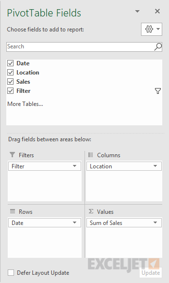
In the pivot table shown, there are three fields in the source data: Date, Sales, and Filter. Filter is a helper column with a formula flagging the last 12 months. The Date field has been grouped by Year and Month:

Formula

The formula used in E5, copied down, is:

=AND(B5>=EOMONTH(TODAY(),-13)+1,B5<EOMONTH(TODAY(),-1))

This formula returns TRUE when a date is greater than or equal to the first day of the month 12 months earlier and when the date is less than the last day of the previous month. The formula uses the AND, TODAY, and EOMONTH functions as explained here.

Steps

1. Add helper column with formula to data as shown
2. Create a pivot table
3. Add Sales as a Value field
4. Add Date as a Row field
5. Group Date by Year and Month
6. Disable subtotals for Year
7. Add helper column as a Filter, filter on TRUE