Pivot table last 4 weeks

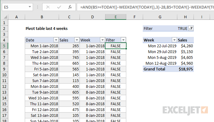
To create a pivot table that shows the last 4 weeks of data (i.e. a rolling 4 weeks), you can add a helper column to the source data to flag records in the last 4 weeks, then use the helper column to filter the data in the pivot table. In the example shown, the current date is August 25, 2019, and the pivot table shows 4 complete previous. When new data is added over time, the pivot table will continue to track the previous 4 weeks based on the current date.

Fields

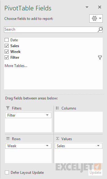
In the pivot table shown, there are four fields in the source data: Date, Sales, Week, and Filter. Filter is a helper column with a formula flagging the last 4 weeks. Week is a helper column that returns the Monday for any given date (for convenience only). Sales is the value field, and Week has been added as a Row field to group by week:

Formula

The formula used in D5 (Week), copied down, is:

=B5-WEEKDAY(B5,3)

This formula returns the Monday of week for any given date.

The formula used in E5 (Filter), copied down, is:

=AND(B5>=TODAY()-WEEKDAY(TODAY(),3)-28,B5<TODAY()-WEEKDAY(TODAY(),3))

This formula checks for dates in the last n weeks. It returns TRUE when a date is in the last 4 complete weeks, and FALSE if not. See the link for a full explanation.

Customizing week count

To customize the weeks displayed, adjust the Filter formula as needed to increase or decrease days. For example, to display the last 6 weeks (42 days), use:

=AND(B5>=TODAY()-WEEKDAY(TODAY(),3)-42,B5<TODAY()-WEEKDAY(TODAY(),3))

Steps

1. Add helper column for Week with the formula above
2. Add helper column for Filter with the formula above
3. Create a pivot table
4. Add Sales as a Value field
5. Add Week as a Row field
6. Set number formatting for Week as desired
7. Add helper column as a Filter, filter on TRUE