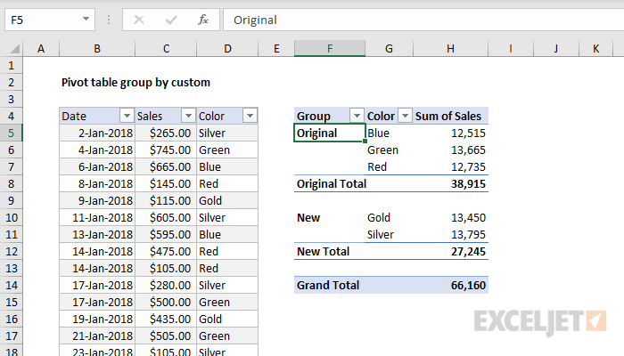
Pivot table group by custom

Pivot tables have a built-in feature to allow manual grouping. In the example shown, a pivot table is used to group colors into two groups: Original and New. Notice these groups do not appear anywhere in the source data.

Fields

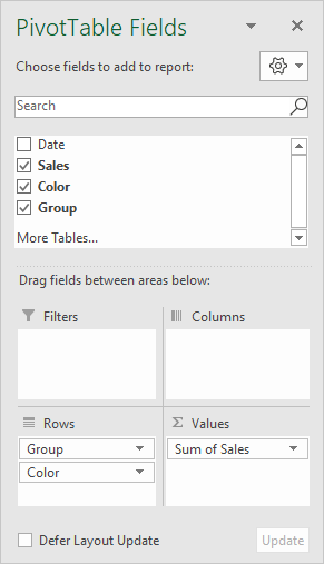
The source data contains three fields: Date, Sales, and Color. A fourth field, Group is created by the grouping process: 

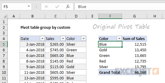
Before grouping, the original pivot table looks like this:

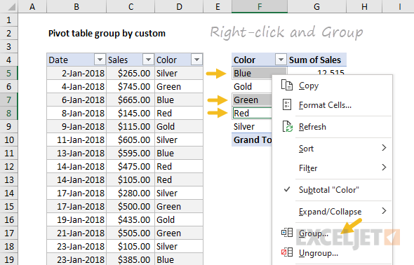
Manual grouping is done by selecting the cells that make up a group. The control key must be held down to allow non-contiguous selections.

With cells selected, right-click and select Group from the menu:

Repeat the process with the second group of items, Gold and Silver. The final two groups are named "Original" and "New".

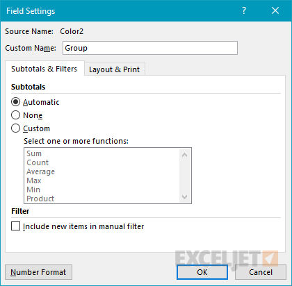
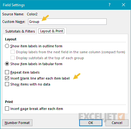
Excel will name the grouping field "Color2". In the example, this field has been renamed "Group":

In addition, the grouping field is configured to insert a blank like after each new group:

Helper column alternative

As an alternative to manual grouping, you can add a helper column to the source data, and use a formula to assign groups. Once you have the grouping labels in the helper column, add the field directly to the pivot table as a row or column field .

Steps

1. Create a pivot table
2. Drag the Color field to the Rows area
3. Drag the Sales field to the Values area
4. Group items manually
   1. Select items
   2. Right-click and Group
   3. Name group as desired
   4. Repeat for each separate group
5. Rename grouping field (Color2) to Group (or as desired)