WEIBULL.DIST Function

The WEIBULL.DIST function calculates values for the Weibull distribution, which is a continuous probability distribution used to model the time until a specified event, such as the failure of a machine part. The Weibull distribution is especially useful in reliability analysis and life data analysis, as it can model increasing, constant, or decreasing failure rates depending on the value of the shape parameter (alpha).

Key features

• Returns either the probability density function (PDF) or the cumulative distribution function (CDF)
• Shape parameter (alpha) controls the failure rate behavior
• Scale parameter (beta) stretches or compresses the distribution
• Can model a wide range of failure behaviors
• All parameters must be positive numbers

WEIBULL.DIST replaces the older WEIBULL function, which is still available for backward compatibility. Microsoft recommends using WEIBULL.DIST for new work.

Table of contents

• Key features
• Example #1 - Light bulb lifetime analysis
• Example #2 - Effect of shape parameter (alpha)
• Example #3 - Effect of scale parameter (beta)
• Example #4 - Cumulative vs. probability density
• Example #5 - Error Conditions
• When to use the Weibull distribution
• Related functions
• Formula definition

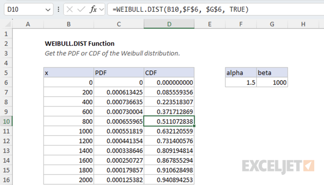
Example #1 - Light bulb lifetime analysis

Suppose you are analyzing the lifetimes of a batch of light bulbs. Historical data suggests that the lifetimes follow a Weibull distribution with a shape parameter (alpha) of 1.5 and a scale parameter (beta) of 1000 hours. You want to know the probability that a randomly selected bulb will fail within 800 hours.

To calculate this probability, use the cumulative distribution function (CDF):

=WEIBULL.DIST(800, 1.5, 1000, TRUE) // returns 0.511

This formula returns the probability that a bulb fails at or before 800 hours. For example, if the result is 0.511, it means there is a 51.1% chance a bulb will fail within 800 hours.

To find the probability that a bulb lasts longer than 800 hours, subtract the CDF from 1:

=1-WEIBULL.DIST(800, 1.5, 1000, TRUE) // returns 0.489

This gives the probability that a bulb survives past 800 hours.

The Weibull distribution is flexible and can model different types of failure rates. In this example, with alpha > 1, the failure rate increases over time, which is typical for aging products.

Example #2 - Effect of shape parameter (alpha)

The shape parameter (alpha) determines the behavior of the failure rate:

• If alpha < 1, the failure rate decreases over time (infant mortality)
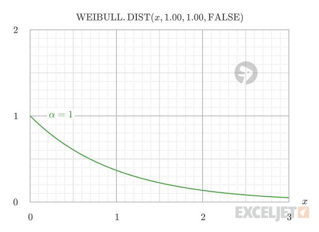
• If alpha = 1, the failure rate is constant (exponential distribution)
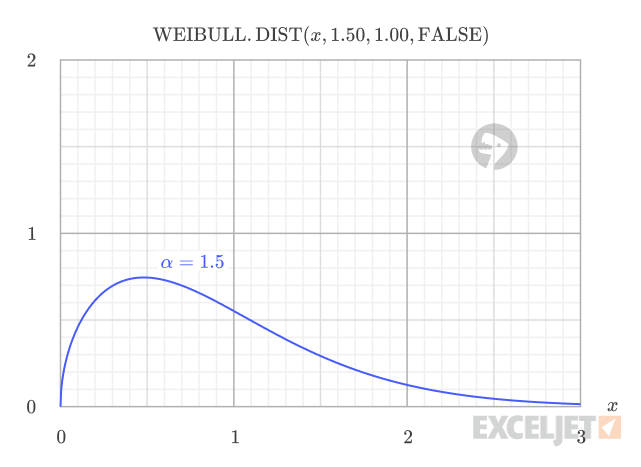
• If alpha > 1, the failure rate increases over time (wear-out failures)

If alpha < 1: Failures are most likely to happen early in the item's life, and those that survive become less likely to fail as time goes on. This is typical for products with early-life defects.

If alpha = 1: The chance of failure is always the same, no matter how long the item has lasted. This models random, unpredictable failures with no aging effect.

If alpha > 1: The risk of failure grows as the item ages, which is common for products that wear out or degrade with use.

Example #3 - Effect of scale parameter (beta)

The scale parameter (beta) stretches or compresses the distribution along the x-axis. In time-based applications, larger values of beta mean the event (e.g., failure) is expected to occur later. The scale parameter typically corresponds to time units such as hours, days, or years in reliability analysis, or distance units such as miles or kilometers for applications like automotive component wear.

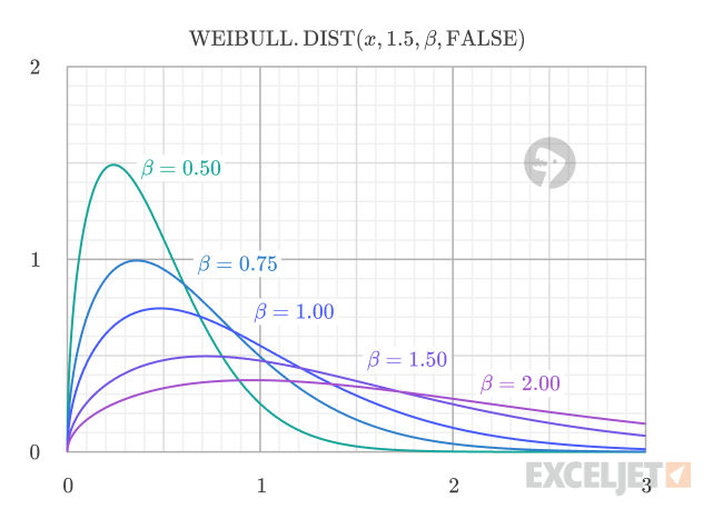
For example, consider different brands of light bulbs with varying quality levels. All follow a Weibull distribution with shape parameter alpha = 2.0 (indicating wear-out failures), but they have different scale parameters representing their expected lifetimes. Compare the probability of failure by 800 hours for different scale parameters:

=WEIBULL.DIST(800, 2.0, 1000, TRUE)   // returns 0.473
=WEIBULL.DIST(800, 2.0, 1500, TRUE)   // returns 0.198
=WEIBULL.DIST(800, 2.0, 2000, TRUE)   // returns 0.095

As beta increases, the probability of failure by 800 hours decreases, indicating longer expected lifetimes for higher-quality bulbs.

Example #4 - Cumulative vs. probability density

The cumulative argument determines whether WEIBULL.DIST returns the cumulative distribution function (CDF) or the probability density function (PDF).

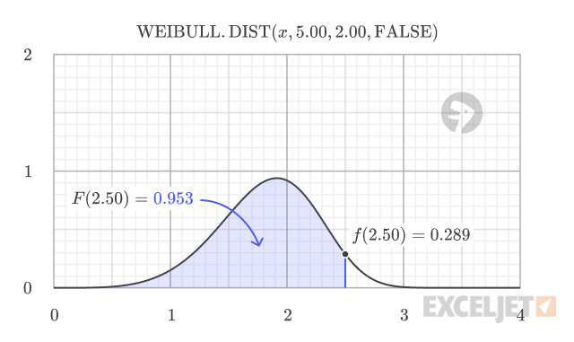
When cumulative is FALSE, the function returns the probability density function (PDF), which indicates the relative likelihood of a random variable taking on a value near a specific point. The PDF value is not a probability itself, but a measure of probability density. For example, at x = 2.5, the PDF value of 0.289 indicates the relative likelihood of failure at that specific point.

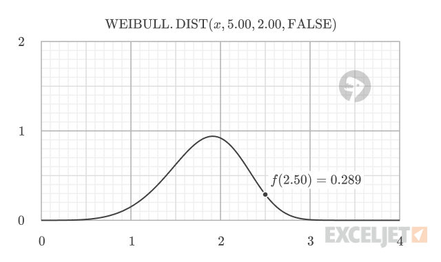
=WEIBULL.DIST(2.5, 5.0, 2.0, FALSE) // returns 0.289 (PDF)

When cumulative is TRUE, the function returns the cumulative distribution function (CDF), which gives the probability of a random variable being less than or equal to a certain value. For example, at x = 2.5, the CDF value of 0.953 means there is a 95.3% probability that a failure will occur by that point.

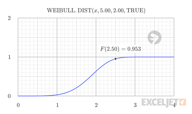
=WEIBULL.DIST(2.5, 5.0, 2.0, TRUE)  // returns 0.953 (CDF)

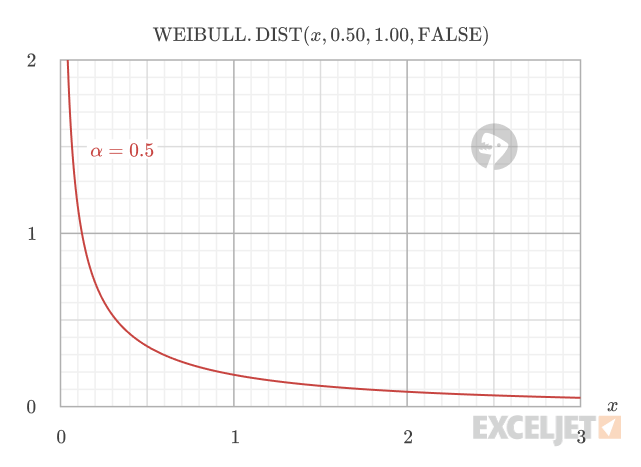
The CDF has a characteristic S-shape, starting at 0 and smoothly increasing toward 1 as x grows larger. The CDF value at any point equals the area under the PDF curve to the left of that point. This relationship is visually demonstrated in the following image, where the total area under the PDF curve is 1.

Using the CDF, you can calculate probabilities for different scenarios. To calculate the probability of an event occurring below a threshold:

=WEIBULL.DIST(threshold, alpha, beta, TRUE)

To calculate the probability of an event occurring above a threshold:

=1 - WEIBULL.DIST(threshold, alpha, beta, TRUE)

To calculate the probability of an event occurring between two thresholds:

=WEIBULL.DIST(upper, alpha, beta, TRUE) - WEIBULL.DIST(lower, alpha, beta, TRUE)

Example #5 - Error Conditions

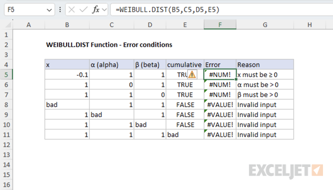
The WEIBULL.DIST function returns the following errors:

• If x < 0, the function returns #NUM! error
• If alpha ≤ 0 or beta ≤ 0, the function returns #NUM! error
• If any argument is non-numeric, the function returns #VALUE! error

The following image shows the error conditions for the WEIBULL.DIST function.

When to use the Weibull distribution

The Weibull distribution is ideal for modeling time-to-failure data in reliability engineering and survival analysis. Its key advantage is the flexible shape parameter (α) that can model different failure patterns:

• α < 1 - Decreasing failure rate (early-life failures)
• α = 1 - Constant failure rate (exponential distribution)
• α > 1 - Increasing failure rate (wear-out failures)

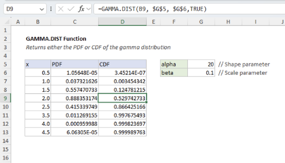
For most reliability analyses, WEIBULL.DIST is preferred over alternatives like GAMMA.DIST, which is better suited for modeling aggregate waiting times rather than time-to-first-failure scenarios.

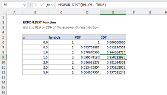
The EXPON.DIST function (Exponential distribution) is a special case of the Weibull distribution when alpha = 1.

Related functions

Excel provides several related functions for probability distributions:

• GAMMA.DIST - Gamma distribution (more general form)
• EXPON.DIST - Exponential distribution (special case of Weibull, alpha = 1)
• CHISQ.DIST - Chi-squared distribution
• LOGNORM.DIST - Log-normal distribution

Formula definition

The formulas for the PDF and CDF of the Weibull distribution are:

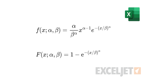
Where:

• f - probability density function
• F - cumulative distribution function
• x - the value at which to evaluate the distribution (must be ≥ 0)
• α (alpha) - the shape parameter of the distribution (must be > 0)
• β (beta) - the scale parameter of the distribution (must be > 0)