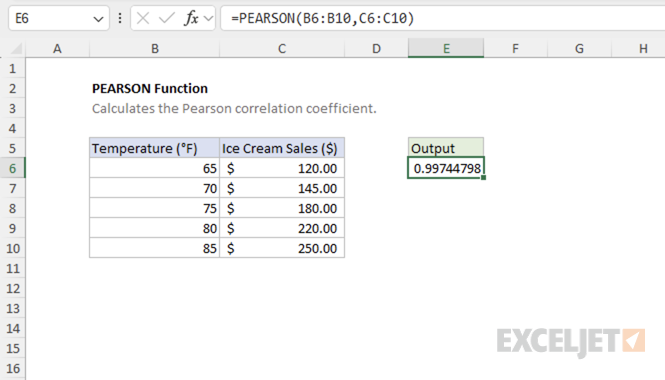
PEARSON Function

The PEARSON function computes the Pearson product-moment correlation coefficient for two arrays of numbers. It quantifies both the strength and direction of a linear relationship, with results ranging from -1 (perfect negative correlation) to 1 (perfect positive correlation).

Key features

• Returns values between -1 and 1 (inclusive)
• Positive values close to 1 indicate a strong positive correlation
• Negative values close to -1 indicate a strong negative correlation
• Values near zero indicate weak or no linear correlation
• Standardized and unit-independent
• Both arrays must have the same number of data points
• Ignores text and logical values; works with numbers only

Note: The PEARSON function is functionally identical to CORREL. Both return the Pearson correlation coefficient.

Table of contents

• Key features
• Example #1 - Strong Positive Correlation
• Example #2 - Strong Negative Correlation
• Example #3 - Weak Correlation
• Example #4 - Edge cases and error handling
• When to use PEARSON
• Formula definition

Example #1 - Strong Positive Correlation

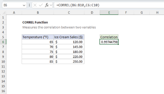
In this example, we'll examine the relationship between temperature (°F) and ice cream sales ($). As temperature increases, ice cream sales tend to increase as well, demonstrating a strong positive correlation.

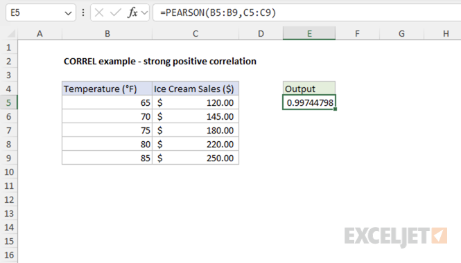
=PEARSON(B5:B9,C5:C9) // returns 0.997447985

The result indicates a strong positive correlation between temperature and ice cream sales.

Example #2 - Strong Negative Correlation

Here we examine the relationship between a car's mileage (miles) and its resale value. As mileage increases, the car's value decreases proportionally, showing a strong negative correlation.

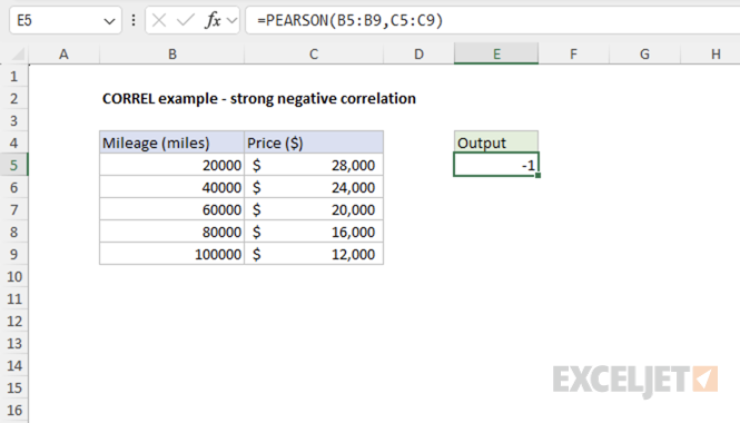
=PEARSON(B5:B9,C5:C9) // returns -1

The result confirms a strong negative correlation between car mileage and its market value.

Example #3 - Weak Correlation

This example illustrates two variables with a weak relationship: daily temperature and coffee sales. While there might be some relationship, it's not very strong.

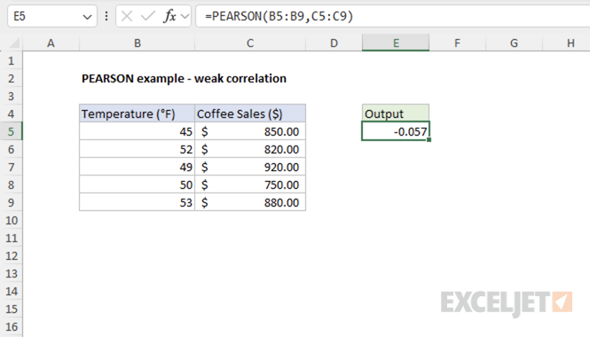
=PEARSON(B5:B9,C5:C9) // returns -0.057

The result close to zero indicates a weak negative correlation between temperature and coffee sales.

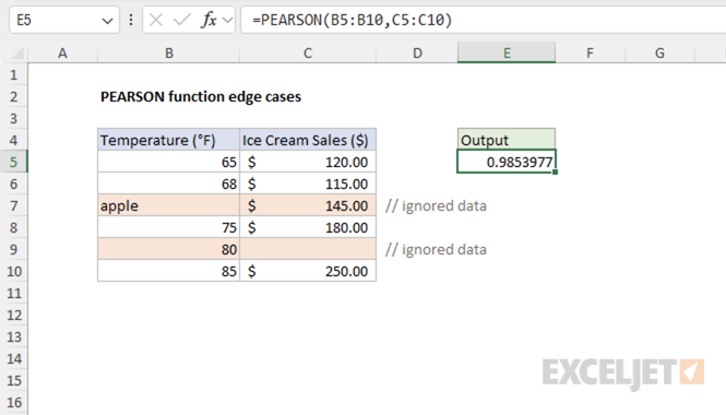
Example #4 - Edge cases and error handling

If either array contains a text value or an empty cell in a given position, PEARSON ignores the pair of data at that position. In the first screenshot below, the arrays contain a text value and an empty cell. These pairs are ignored, and the function calculates the correlation using only the remaining numeric pairs.

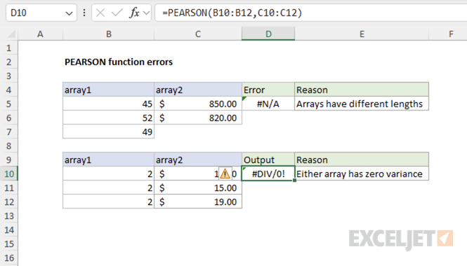
The second screenshot demonstrates two common errors:
- #DIV/0! error: This occurs when either array has zero variance (all values are identical), so the correlation is undefined.
- #N/A error: This occurs when the arrays have different lengths.

When to use PEARSON

Use PEARSON when you need to measure the linear relationship between two sets of numerical data in Excel. Choose PEARSON (or CORREL) when you want a standardized, unit-independent measure of correlation. Use covariance functions (COVARIANCE.P or COVARIANCE.S) if you need to know the magnitude of change as well as direction.

PEARSON only measures linear relationships; it does not detect non-linear associations.

Key advantages

• Standardized scale (-1 to +1) for easy interpretation
• Unit-independent, allowing comparison across different measurement scales
• Indicates both direction and strength of relationship
• Widely used and recognized in statistics

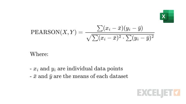
Formula definition

The PEARSON function uses the following formula: