GROWTH Function

The GROWTH function calculates exponential growth predictions based on existing data points. It fits an exponential curve (y = b*m^x) to your known data and then uses that curve to predict future values. GROWTH is particularly useful for forecasting trends that follow exponential patterns, such as population growth, compound interest, or viral spread.

Key features

• Fits an exponential curve to existing data points
• Predicts values based on the fitted curve
• Can be used for both interpolation and extrapolation

GROWTH assumes your data follows an exponential pattern y = b*m^x or y = m^x . If your data follows a different pattern (linear, logarithmic, etc.), consider using the related functions listed above instead.

Table of contents

• Key features
• Example #1 - Basic GROWTH calculation
• Example #2 - Predict future and past values
• Example #3 - Interpolate fractional values
• Example #4 - Using the const parameter
• Example #5 - Error Conditions
• How it works
• Notes

Example #1 - Basic GROWTH calculation

The GROWTH function takes up to four arguments in this syntax:

=GROWTH(known_y, [known_x], [new_x], [const])

In its simplest form, you can use GROWTH with known y-values and x-values, plus new x-values for prediction. Here is an example:

=GROWTH({100,150},{1,2},{2,3,4}) // spills {150,225,337.5}

The function fits an exponential curve to your data and returns predicted values for the specified new x-values.

Example #2 - Predict future and past values

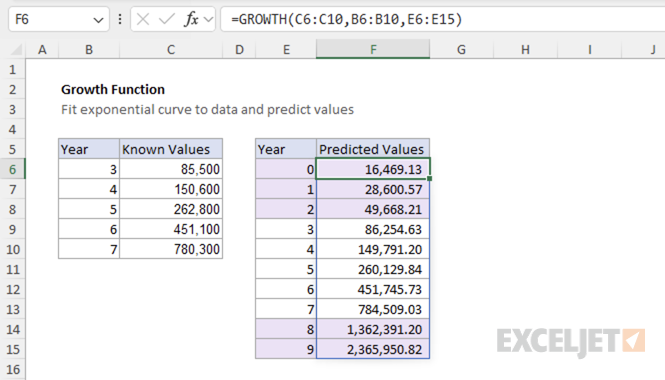
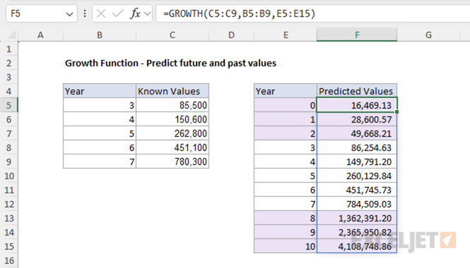
In the example below, we have data for years 3-7 and want to predict values for years 0-10 (both past and future). The formula in cell F5 is:

=GROWTH(C5:C9,B5:B9,E5:E15)

The GROWTH function:
1. Fits an exponential curve to the known data (years 3-7)
2. Uses that curve to predict values for the new x-values
3. Returns the predicted values as an array, showing both past predictions (years 0-2) and future predictions (years 8-10)

Note: The predicted values for the known data points (years 3-7) may differ slightly from the actual values shown in the data. This is because GROWTH fits the best exponential curve to all the data points, and the curve may not pass exactly through each individual point. The function prioritizes finding the overall exponential trend rather than matching each data point exactly.

Example #3 - Interpolate fractional values

In this example, we use GROWTH to interpolate values between existing data points, including fractional years. Imagine a business that has enjoyed exceptional growth over the past 5 years and wants to track their progress quarterly to ensure they're on track for the next year. We have data for years 3-7 and want to find values for each quarter between years 6 and 8. The fractional years represent quarters:

• 6.00 = Start of year 6 (Q1)
• 6.25 = End of Q1 in year 6
• 6.50 = End of Q2 in year 6
• 6.75 = End of Q3 in year 6
• 7.00 = End of Q4 in year 6
• And so on...

The formula in cell F5 is:

=GROWTH(D5:D9,C5:C9,E5:E13)

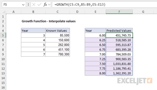
The GROWTH function:
1. Fits an exponential curve to the known data points (years 3-7)
2. Uses that curve to calculate values for the specified x-values
3. Returns the interpolated values as an array, showing predictions for fractional time periods

Example #4 - Using the const parameter

The const parameter controls whether the exponential curve starts at one or some base amount at x=0. For example, when const=TRUE (the default behavior), GROWTH calculates the optimal starting value by fitting the best exponential curve of the form y = b*m^x, where both b and m are calculated to best fit your data:

=GROWTH(C5:C9,B5:B9,E5:E15,TRUE)

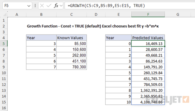
In this case, the function fits the exponential curve to the data, where the starting value is b = 16,469.13 and the growth rate is m ≈ 1.737.

In contrast, when const=FALSE, GROWTH sets the constant b to equal 1, fitting the curve y = m^x:

=GROWTH(C5:C9,B5:B9,E5:E15,FALSE)

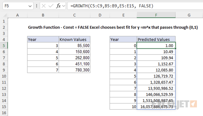
With const=FALSE, the function sets b = 1, so the curve passes through (0,1), and calculates the value for m (growth rate) that best fits the data. For this data, setting const to FALSE does not produce a better fit. The constraint of forcing the curve through (0,1) creates a much steeper growth rate that overestimates the actual values by orders of magnitude.

You should use const=FALSE when it makes sense for the exponential curve to start at 1. For example, when working with relative growth rates where the starting point is naturally one.

Example #5 - Error Conditions

The GROWTH function returns #NUM! if any of the known_y values are zero or negative.

=GROWTH({0,4,8},{1,2,3}) // returns #NUM!

The GROWTH function returns #VALUE! if any arguments are non-numeric.

=GROWTH({"1",4,8},{1,2,3}) // returns #VALUE!

The Growth function returns #REF! if the known_x and new_x arrays have different lengths.

=GROWTH({2,4,8},{1,2}) // returns #REF!

How it works

The GROWTH function fits an exponential curve to your data and returns predicted values for the specified new x-values. The curve is defined by the equation:

y = b * m^x

Where:
- b is the base amount
- m is the growth multiplier
- x is the independent variable (time)

To calculate the exponential curve manually, we use an equivalent form that makes the calculations easier:

y = b * EXP(k * x)

Where:
- EXP is the Exponential function
- k is the growth coefficient (related to m by m = EXP(k))
- b and x are the same as above

This form makes it easier to calculate the growth coefficient and base amount manually using Excel's SLOPE and INTERCEPT functions.

Step 1: Calculate growth coefficient k:

To calculate the growth coefficient k, we calculate the natural log of the y-values and then use the SLOPE function to calculate the slope of the line.

=SLOPE(ln_y_values, x_values) // returns k

Step 2: Calculate base amount b:

To calculate the base amount b, we use the INTERCEPT function to calculate the y-intercept of the line, then apply the exponential function.

=EXP(INTERCEPT(ln_y_values, x_values)) // returns b

Step 3: Predict values:

To predict values using the exponential curve, we use the formula:

=b * EXP(k * new_x)

This returns the same results as the GROWTH function. For example, given data that starts at 10 and doubles each time (10, 20, 40, 80, 160, 320, 640), we can calculate the exponential curve manually as shown in the screenshot below.

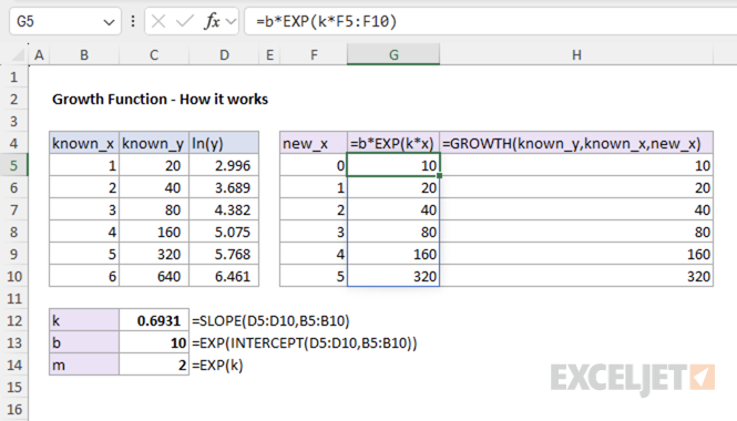
Step 4: (Optional) Calculate growth multiplier m:

If you prefer to write the exponential curve in the form y = b*m^x instead of y = b * EXP(k * x), you can calculate the growth multiplier m by applying the exponential function to the growth coefficient k:

=EXP(k) // returns m

Then you can write the prediction formula as:

=b * m^x

This gives you the same exponential curve, just expressed in a different form.

Notes

• GROWTH is an array function that returns multiple values when you specify multiple new_x values.
• In Excel 365, simply press Enter to enter the formula. In Excel 2019 and earlier, use Ctrl+Shift+Enter for array formulas.
• When using GROWTH with a single new_x value, it returns a single result and behaves like a regular function.