Summary
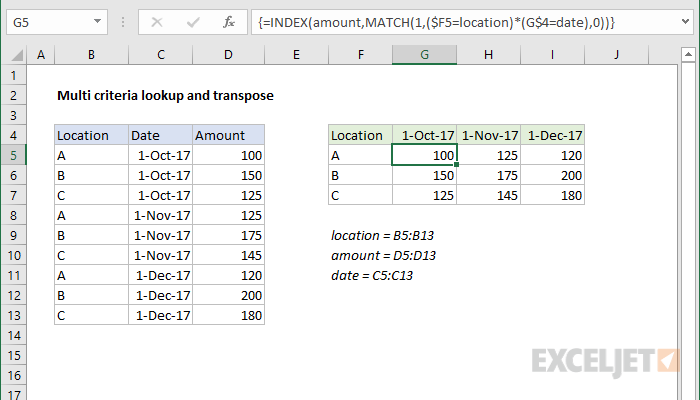
To perform a multi-criteria lookup and transpose results into a table, you can use an array formula based on INDEX and MATCH. In the example shown, the formula in G5 is:
{=INDEX(amount,MATCH(1,($F5=location)*(G$4=date),0))}
Note this formula is an array formula and must be entered with control + shift + enter.
This formula also uses three named ranges: location = B5:B13, amount = D5:D13, date = C5:C13
Generic formula
{=INDEX(rng1,MATCH(1,($A1=rng2)*(B$1=rng3),0))}
Explanation
The core of this formula is INDEX, which is retrieving a value from the named range "amount" (B5:B13):
=INDEX(amount,row_num)
where row_num is worked out with the MATCH function and some boolean logic:
MATCH(1,($F5=location)*(G$4=date),0)
In this snippet, the location in F5 is compared with all locations, and the date in G4 is compared with all dates. The result in each case is an array of TRUE and FALSE values. When these arrays are multiplied together, the math operation coerces the TRUE and FALSE values to one's and zeros, so that the lookup array going into MATCH looks like this:
{1;0;0;0;0;0;0;0;0}
MATCH is set up to match 1 as an exact match, and returns the position to INDEX as a row number. The number 1 works for the lookup value because the array now contains only 1's and 0's, as shown above.
F5 and G4 are entered as mixed references so that the formula can be copied through the table without modification.
Transpose with paste special
If you just need to transpose a table one time, don't forget you can use paste special.